Topics to cover

I had two major sections in the Appendix of last week’s post:

1. “Multiple matrix transformations”
2. “Potential improvements” (where I mostly describe limitations around visualizing rotations)

This post expands on these topics.

animatrixr and multiple matrix transformations

Sanderson discusses the value in sometimes decomposing a matrix transformation and thinking of its parts sequentially. I created a toy package animatrixr for building chained matrix transformations that can then be animated using gganimate¹.

The function animatrixr::add_transformation() lets you chain together matrix transformations with R’s pipe operator %>%.

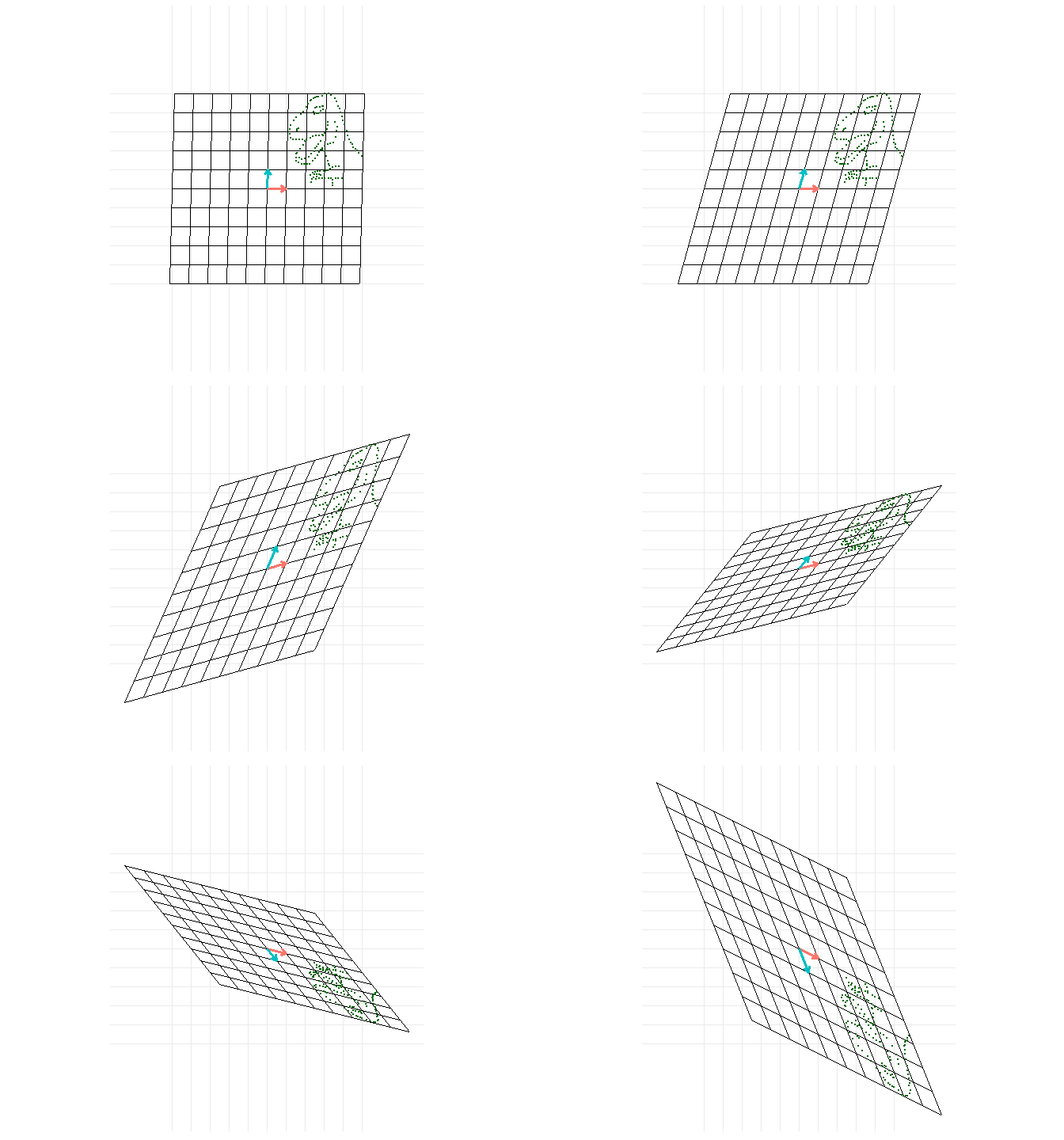
For example, let’s consider three matrix transformations: horizontal sheer –> vertical sheer –> reflection across x-axis:

library(dplyr)

if (!requireNamespace("animatrixr")) devtools::install_github('brshallo/animatrixr')
library(animatrixr)

sheer_horizontal <- tribble(~ x, ~ y,
                      1, 0.5,
                      0, 1) %>%
  as.matrix()

sheer_vertical <- tribble(~ x, ~ y,
                      1, 0,
                      0.5, 1) %>%
  as.matrix()

reflect_x <- tribble(~ x, ~ y,
                      1, 0,
                      0, -1) %>%
  as.matrix() 

Now let’s visualize the transformations being applied sequentially:

matrix(c(1,0,0,1), nrow = 2) %>% 
  add_transformation(sheer_horizontal) %>% 
  add_transformation(sheer_vertical) %>% 
  add_transformation(reflect_x, 
                     seq_fun = animatrixr::seq_matrix_l,
                     n_frames = 40) %>% 
  animate_matrix(datasaurus = TRUE)

add_transformation() explicitly creates in-between frames for a given transformation. The seq_fun argument allows you to define the interpolation method, for example whether the coordinates should (during the animation) follow a linear path (default) or the angle of a rotation.

It would be nice to add-in functionality where the final transformation object could then be added to layers of a ggplot (though I’ve done nothing towards this except add an argument in animatrixr::animate_matrix() for displaying the datasauRus).

(Warning: animatrixr is severely limited, as discussed in the Appendix and in package documentation. However you can find it at the “brshallo/animatrixr” repo on my github page.)

Visualizing rotations

The seq_fun argument within add_transformation() specifies frames in-between the start and end states after a matrix transformation. By default it uses animatrixr::seq_matrix_l which changes in-between coordinates linearly (as does gganimate²).

Let’s look at a rotation where the in-between coordinates are interpolated linearly:

rotate_90 <- tribble(~ x, ~ y,
                        cos(pi / 2), -sin(pi / 2),
                        sin(pi / 2), cos(pi / 2)) %>%
  as.matrix()

matrix(c(1,0,0,1), nrow = 2) %>% 
  add_transformation(rotate_90) %>% 
  animate_matrix(datasaurus = TRUE)

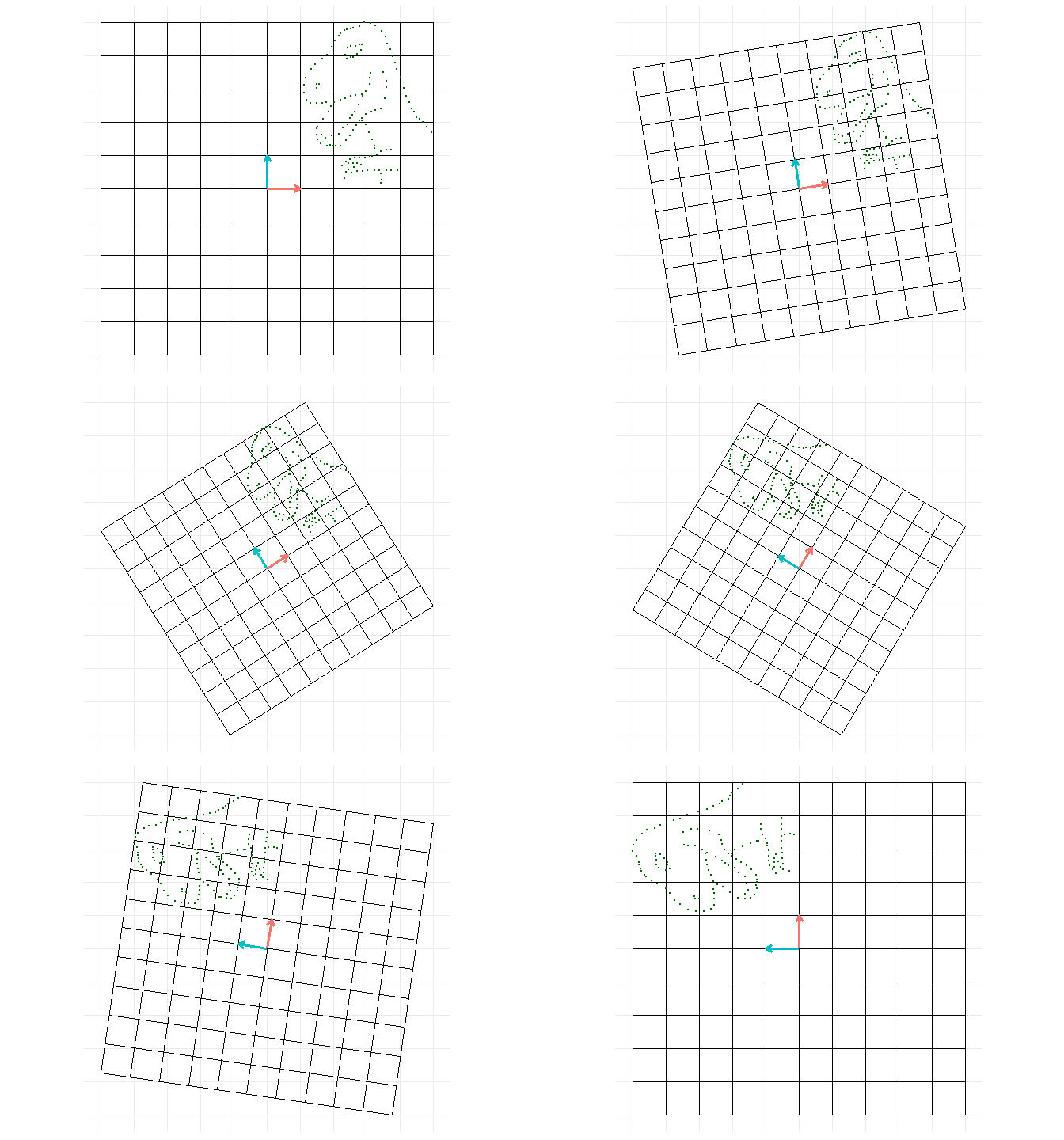
Linear interpolation makes the rotation transformation appear scrunched during the animation (from how we intuitively think of a rotation) as the coordinate points take a straight line path to their positions after applying the transformation³.

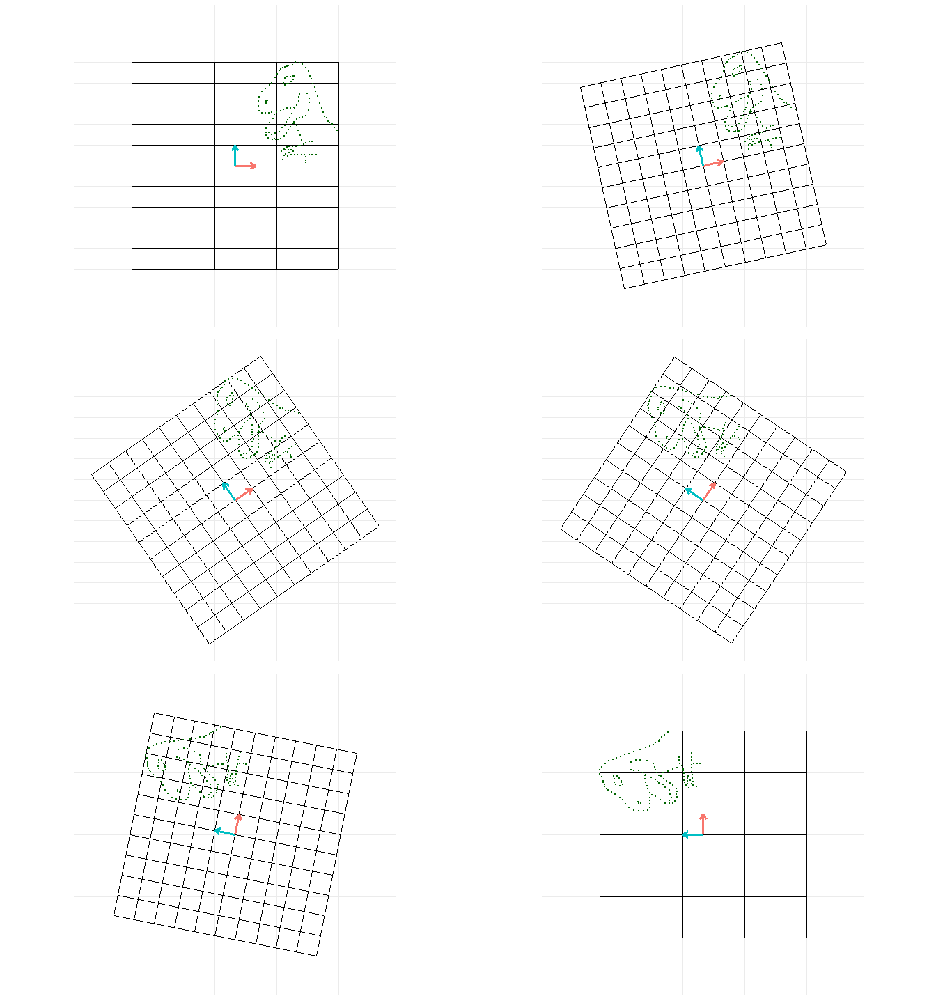
To make the in-between coordinates instead follow the angle of rotation we could change the seq_fun from animatrixr::seq_matrix_l to animatrixr::seq_matrix_lp.

matrix(c(1,0,0,1), nrow = 2) %>% 
  add_transformation(rotate_90, seq_fun = animatrixr::seq_matrix_lp) %>% 
  animate_matrix(datasaurus = TRUE)

During the rotation portion of the animation gganimate is still tweening images linearly, however the frames add_transformation() creates are now following along the angle of rotation of the transformation. Hence the animation ends-up approximating a curved path.

However, seq_matrix_lp() needs improvement and was just set-up to work for toy examples – it really only looks ‘right’ if doing rotations off of \[ \left(\begin{array}{cc} 1 & 0\\0 & 1 \end{array}\right)\] See Showing rotations in the Appendix for additional detail on how this is set-up and the various limitations with animatrixr.

Happy animatrixing!

# animatrixr::rotation_matrix() is helper function for creating matrix
# transformations of rotations
matrix(c(1,0,0,1), nrow = 2) %>% 
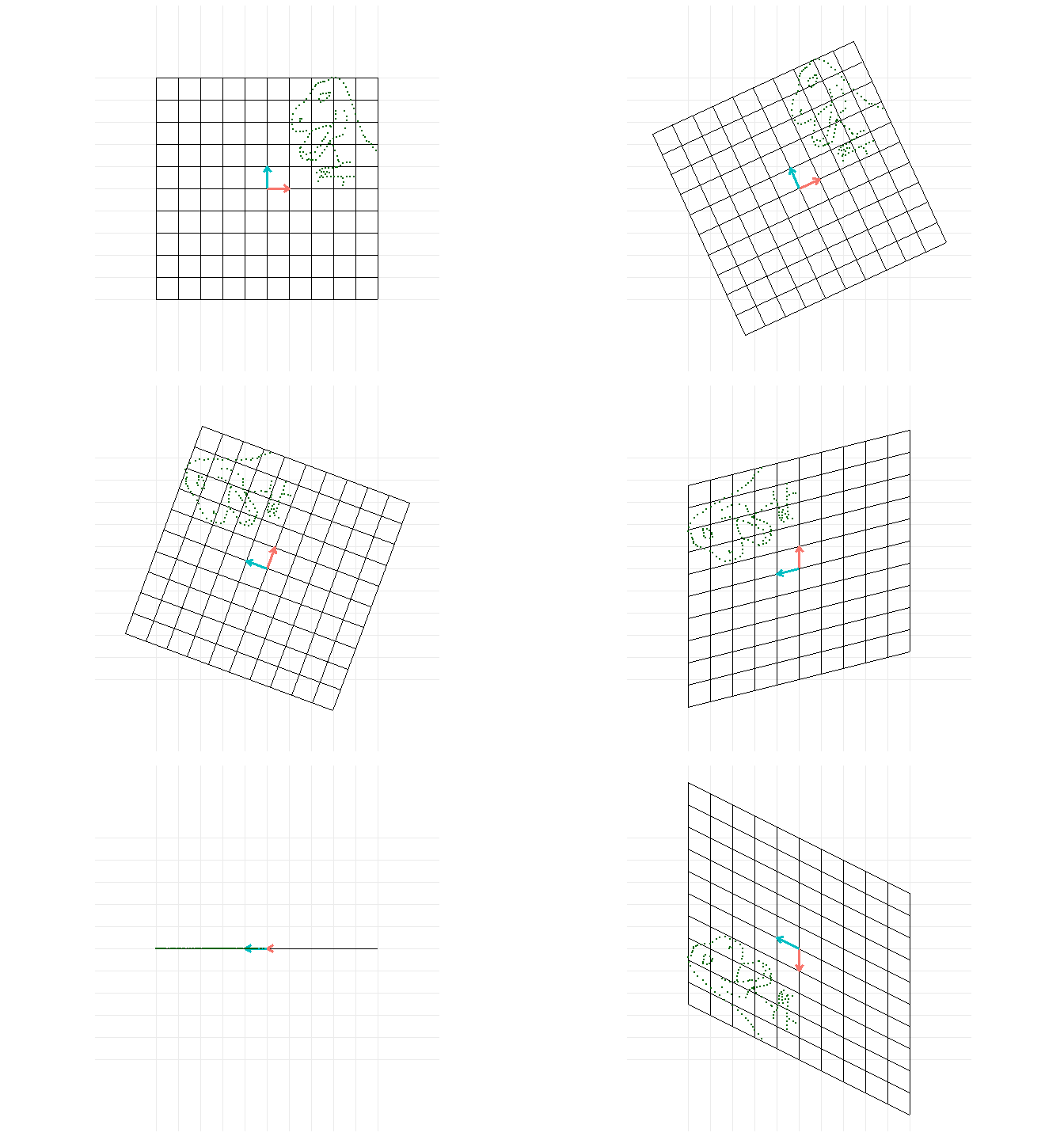
  add_transformation(animatrixr::rotation_matrix(pi / 2),
                     seq_fun = animatrixr::seq_matrix_lp) %>% 
  add_transformation(matrix(c(1, 0.5, 0, 1), nrow = 2)) %>% 
  add_transformation(matrix(c(1, 0, 0, -1), nrow = 2)) %>% 
  animate_matrix(datasaurus = TRUE)

Appendix

transformation_matrix <- sheer_vertical %*% animatrixr::rotation_matrix(pi/4)

matrix(c(1,0,0,1), nrow = 2) %>% 
  add_transformation(transformation_matrix, seq_fun = seq_matrix_rotate_first) %>% 
  animate_matrix(datasaurus = TRUE)