This post contains solutions to FiveThirtyEight’s two riddles released 2020-02-14, Riddler Express and Riddler Classic. I created a toy package animatrixr to help with some of the visualizations and computations for my solutions1.
Riddler express
The riddle:
Riddler City is a large circular metropolis, with countless square city blocks that each have a side length of 1 km. A small section of the city, composed of 36 blocks, is shown in the diagram below:
At the very center of the city lies Riddler City Hall. Its many employees all walk to and from work, and their homes are evenly scattered across the city. The sidewalks they walk along have always been adjacent to the streets — but that may be changing. Recently, several city hall employees submitted a petition, requesting that the sidewalks should no longer lie alongside the streets. Instead, they want the sidewalks to cut diagonally across the city, connecting nearby street intersections. These proposed sidewalks are represented by the thicker blue lines in the diagram below:
The mayor of Riddler City has tasked you with resolving this dispute in a mathematical manner. She would like you to answer the following question: What fraction of the city hall employees would have a shorter walk home (that is, to the street intersection nearest to their home) if the city replaced its traditional sidewalks with these diagonal sidewalks?
– Zach Wissner-Gross, “Can You Solve this Rather Pedestrian Puzzle,” FiveThirtyEight
My approach:
I. Create hypothetical simulation of city
II. For each scenario, calculate Manhattan Distances from center for all points
III. Make distances comparable by scaling by unit length of a city block
IV. Compare distances between scenarios for all points; compute proportion that have shorter path with new diagonal sidewalks
I. Create hypothetical city
I first created a hypothetical 100 unit diameter version of this city2. I added residences at every point on a 100x100 grid and then removed those points that had a euclidean distance3 greater than 50 units from the center.
library(tidyverse)
library(animatrixr)
radius <- 50
df_start <- crossing(x = -radius:radius, y = -radius:radius) %>%
#Removes points with euclidian distance from center > radius:
filter(sqrt(x^2 + y^2) <= radius)II. Calculate Manhattan Distances
For both scenarios, we need to calculate the Manhattan length4 between the origin and every point. To calculate the Manhattan length on the new scenario, we first need to find what the residence’s coordinates would be in the new sidewalk grid. The new coordinate system could be thought of simply as a rotated and shrunken version of the existing grid5, which can be represented as applying the matrix transformation:
\[ M = \left(\begin{array}{cc} 0.5 & -0.5\\0.5 & 0.5 \end{array}\right)\]
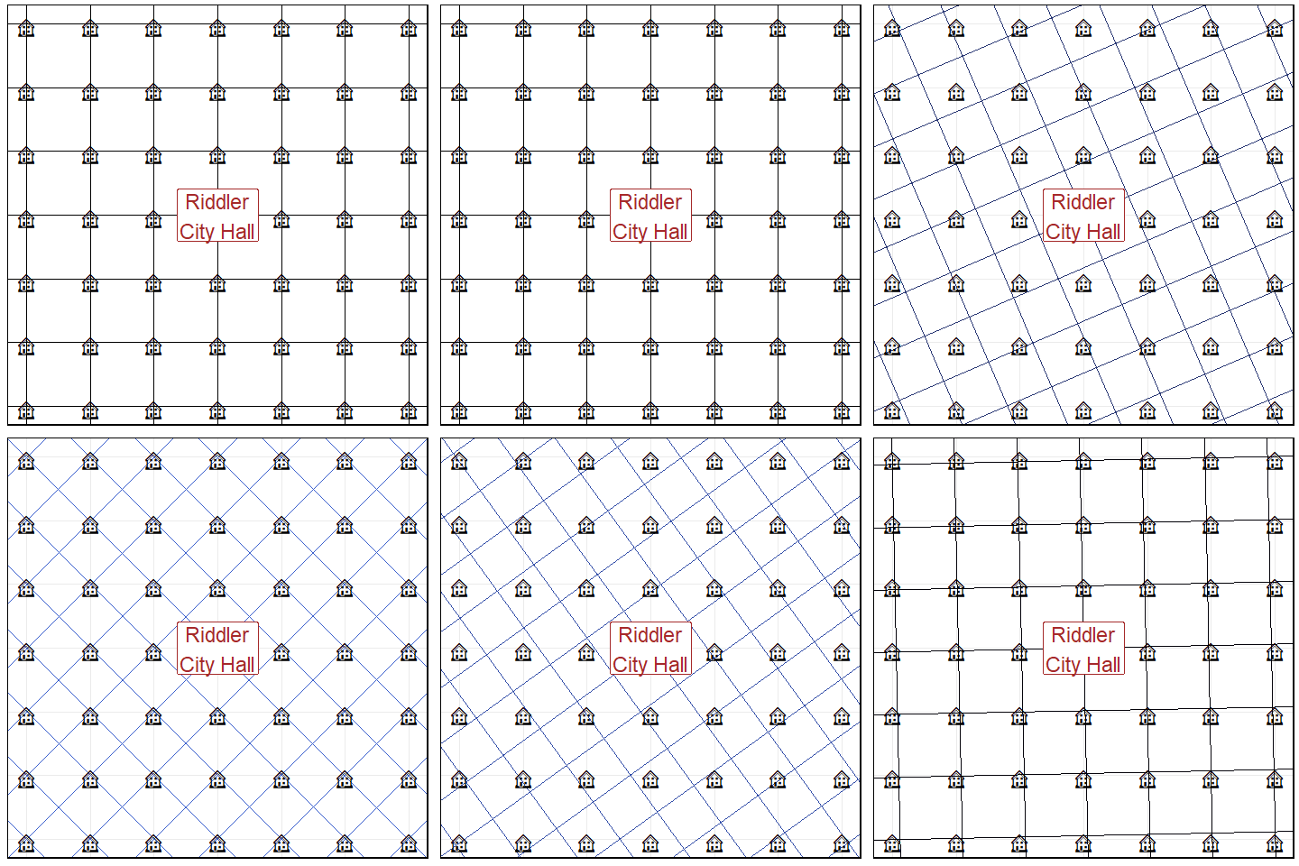
(See Transform city, pretty in the Appendix to view the code used to create the above visualization.)
Our residences are not changing locations, they would just have different coordinates specific to the new sidewalks – hence we will actually apply the inverse6 of this transformation to our starting coordinates. This will give us the position of our residences on the new (transformed) coordinate grid.
\[ M^{-1} = \left(\begin{array}{cc} 1 & 1\\-1 & 1 \end{array}\right)\]
df_trans <- df_start %>%
  mutate(x_trans = x,
         y_trans = y) %>%
  # x_trans, y_trans represent the coordinates on the new plane
  transform_df_coords(x_trans, y_trans, m = matrix(c(1, -1, 1, 1), nrow = 2))
We will then calculate the Manhattan lengths of the points on both the new and old coordinate systems – which (because we are comparing distance from the origin: 0,0) can be computed as: \(Manhattan\;Length = |x| + |y|\).
df_units <- df_trans %>%
  mutate(a_units = abs(x) + abs(y),
         b_units = abs(x_trans) + abs(y_trans))
IV: Multiply Manhattan lengths by length of a block:
The length of a block under the new and old scenarios are different (new diagonal sidewalks have shorter blocks), hence our current Manhattan lengths are not comparable. If we set the length of a single block on the original coordinate system as being 1 unit, then you can use the Pythagorean Theorem to find that the length of a block on the new sidewalks would be \(\frac{\sqrt{2}}{2}\). We simply multiply our Manhattan lengths in each of our scenarios by their respective unit lengths (either 1 or ~0.7071).
df_dists <- df_units %>%
  mutate(a_dist = 1 * a_units,
         b_dist = (sqrt(2) / 2) * b_units)
The scaled distances can now be compared.
V. Aggregate proportion difference:
Finally, we compute the proportion that have a shorter distance under the new sidewalks compared to the old sidewalks:
df_dists %>%
  summarise(prop_shorter = (sum(b_dist < a_dist)/ n()) %>% round(2)) %>%
knitr::kable()| prop_shorter |
|---|
| 0.5 |
Riddler express solution: new diagonal sidewalks would be faster for 50% of people.
Let’s visualize which resident’s the new sidewalks would be faster for:
df_dists %>%
  mutate(diagonal_faster = b_dist < a_dist) %>%
  ggplot(aes(x = x, y = y))+
  geom_point(aes(colour = diagonal_faster))+
  coord_fixed()+
  ggforce::theme_no_axes()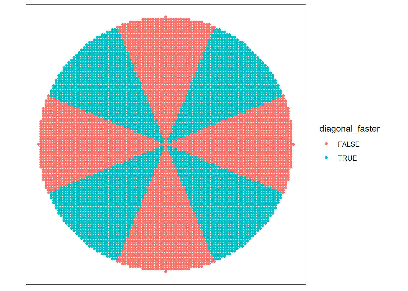
Riddler classic
The riddle:
From David Lewis comes an additional, original twist on Riddler City’s urban planning:
The mayor ultimately decided not to pursue diagonal sidewalks, but the petitioners haven’t given up yet. One of them recently visited Barcelona and was inspired by its octagonal city blocks.
Now, there’s a second petition on the mayor’s desk, asking that the grid layout of the city’s sidewalks be replaced with an octagonal pattern, represented by the thicker blue lines in the diagram below:
Under this second proposal, now what fraction of the employees would have a shorter walk home if the city replaced its traditional sidewalks with these new sidewalks?
– Zach Wissner-Gross, “Can You Solve this Rather Pedestrian Puzzle,” FiveThirtyEight
My approach:
The Barcelona distance is just a combination of the Manhattan lengths of both the original and diagonal sidewalk grids (though with the unit lengths scaled differently)7. The unit lengths8 for the horizontal and diagonal components will depend on what proportion9 of a side is horizontal vs diagonal (corresponding with the original vs transformed grid from the Riddler Express solution)10.
We can define our relevant side lengths as a function of x:
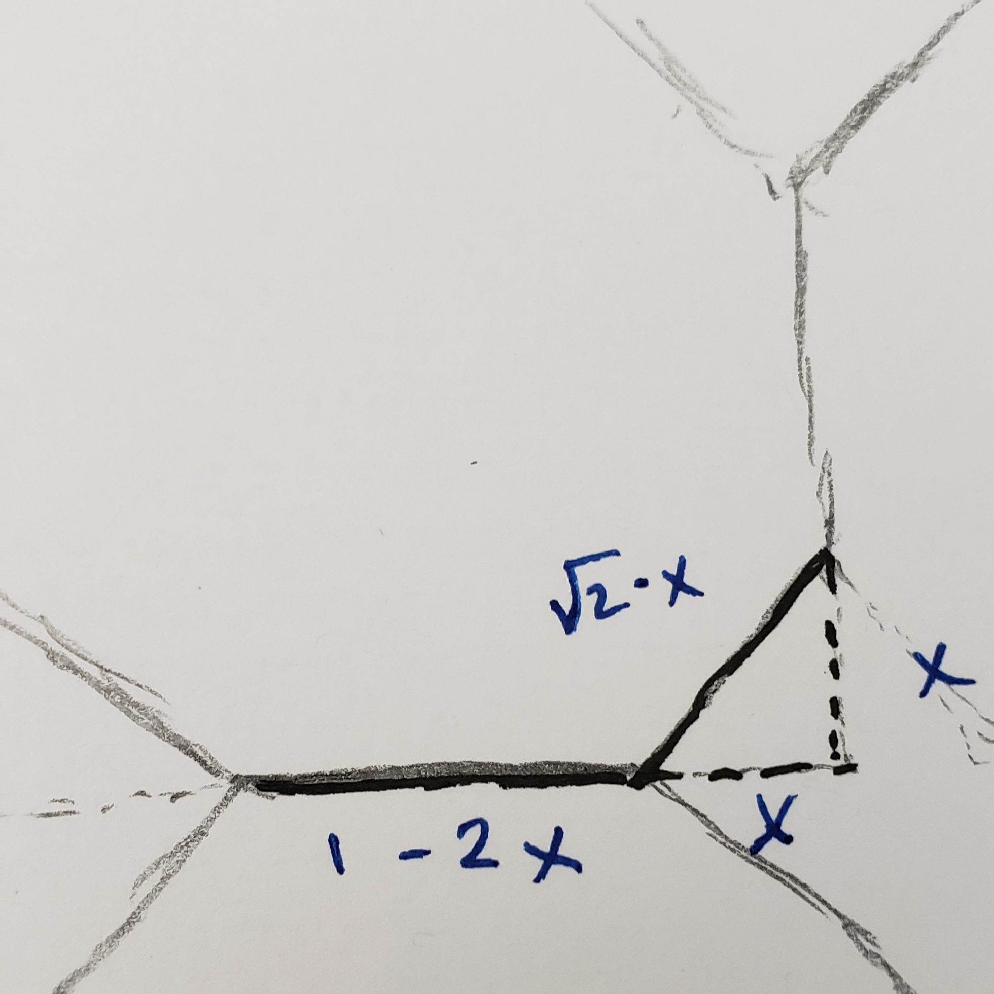
\[x : \frac{inverse\;of\;proportion\;horizontal}{2},\] \[0 < x < 0.5\] \[diagonal\;length = \sqrt{2}x\] \[horizontal\;length = 1 - 2x\]
I’ll start by setting x = 0.25. Hence the Manhattan length of our horizontal component will be scaled by \(\frac{1}{2}\), and our diagonal component will be scaled by \(\frac{\sqrt{2}}{4}\). After scaling our components, we simply add them together to get our Barcelona distance11 12.
x <- 0.25
side_length <- 1 - 2*x
side_length_trans <- sqrt(2)*x

df_dists_abc <- df_dists %>%
  mutate(c_dist_a = a_units * side_length,
         c_dist_b = b_units * side_length_trans,
         c_dist = c_dist_a + c_dist_b)
Finally, for all points, we compare the travel distance on the new Barcelona grid compared to on the original horizontal grid and compute the percentage that have a shorter distance under the new sidewalks.
df_dists_abc %>%
  summarise(prop_shorter = (sum(c_dist < a_dist)/ n()) %>% round(2)) %>%
knitr::kable()| prop_shorter |
|---|
| 0.5 |
In the case (when x is set to 0.25) we see the proportion that is closer to City Hall (i.e. the center of our city13) is again 50%.
If we visualize in which locations the new Barcelona sidewalks have a shorter travel distance, we will see a similar result to that found in the Riddler Express solution.
df_dists_abc %>%
  mutate(barcelona_faster = c_dist < a_dist) %>%
  ggplot(aes(x = x, y = y))+
  geom_point(aes(colour = barcelona_faster))+
  coord_fixed()+
  ggforce::theme_no_axes()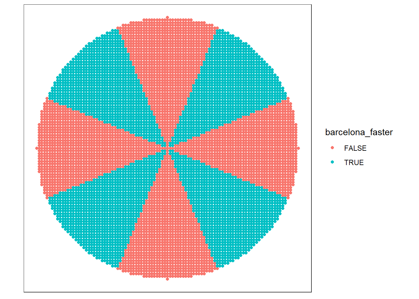
We need to verify that ‘50% have a shorter walk’ is our solution regardless of what we set for x.
To accomplish this, I wrote a function summarise_proportion(), that will output the ‘Proportion Barcelona sidewalk distance is shorter’ across any given x between 0 and 0.5 (the possible values of x).
summarise_proportion <- function(x, df_start = df_dists, out_data = FALSE){

  x <- 0.25
  side_length <- 1 - 2*x
  side_length_trans <- sqrt(2)*x

  df_dists_out <- df_dists %>%
    mutate(c_dist_a = a_units * side_length,
           c_dist_b = b_units * side_length_trans,
           c_dist = c_dist_a + c_dist_b)

  if(out_data) return(df_dists_out)

  df_dists_out %>%
    summarise(prop_shorter = (sum(c_dist < a_dist)/ n())) %>%
    pluck("prop_shorter")
}
Specifically I evaluated this ‘proportion shorter’ for x set to each of \(0.01, 0.05, 0.09, ... 0.49\).
x_vec <- seq(from = 0.01, to = 0.49, by = 0.04)

df_summary <- tibble(x = x_vec) %>%
  mutate(prop_shorter = map_dbl(x, summarise_proportion, df_start = df_dists) %>% round(2))

df_summary %>%
knitr::kable()| x | prop_shorter |
|---|---|
| 0.01 | 0.5 |
| 0.05 | 0.5 |
| 0.09 | 0.5 |
| 0.13 | 0.5 |
| 0.17 | 0.5 |
| 0.21 | 0.5 |
| 0.25 | 0.5 |
| 0.29 | 0.5 |
| 0.33 | 0.5 |
| 0.37 | 0.5 |
| 0.41 | 0.5 |
| 0.45 | 0.5 |
| 0.49 | 0.5 |
For each of these, the new ‘Barcelona grid’ is faster for 50% of people.
Appendix
Time to center
Visualize the distance to the center based on where people are in the city for each of the potential city grids.
df_dists_abc %>%
  select(x, y, a_dist, b_dist, c_dist) %>%
  pivot_longer(cols = c(a_dist, b_dist, c_dist), names_to = "grid", values_to = "distance") %>%
  mutate(grid = fct_recode(grid,
                           "rectangular" = "a_dist",
                           "diagonal" = "b_dist",
                           "barcelona.25" = "c_dist")) %>%
  ggplot(aes(x = x, y = y, colour = distance))+
  geom_point()+
  facet_wrap(~grid)+
  coord_fixed()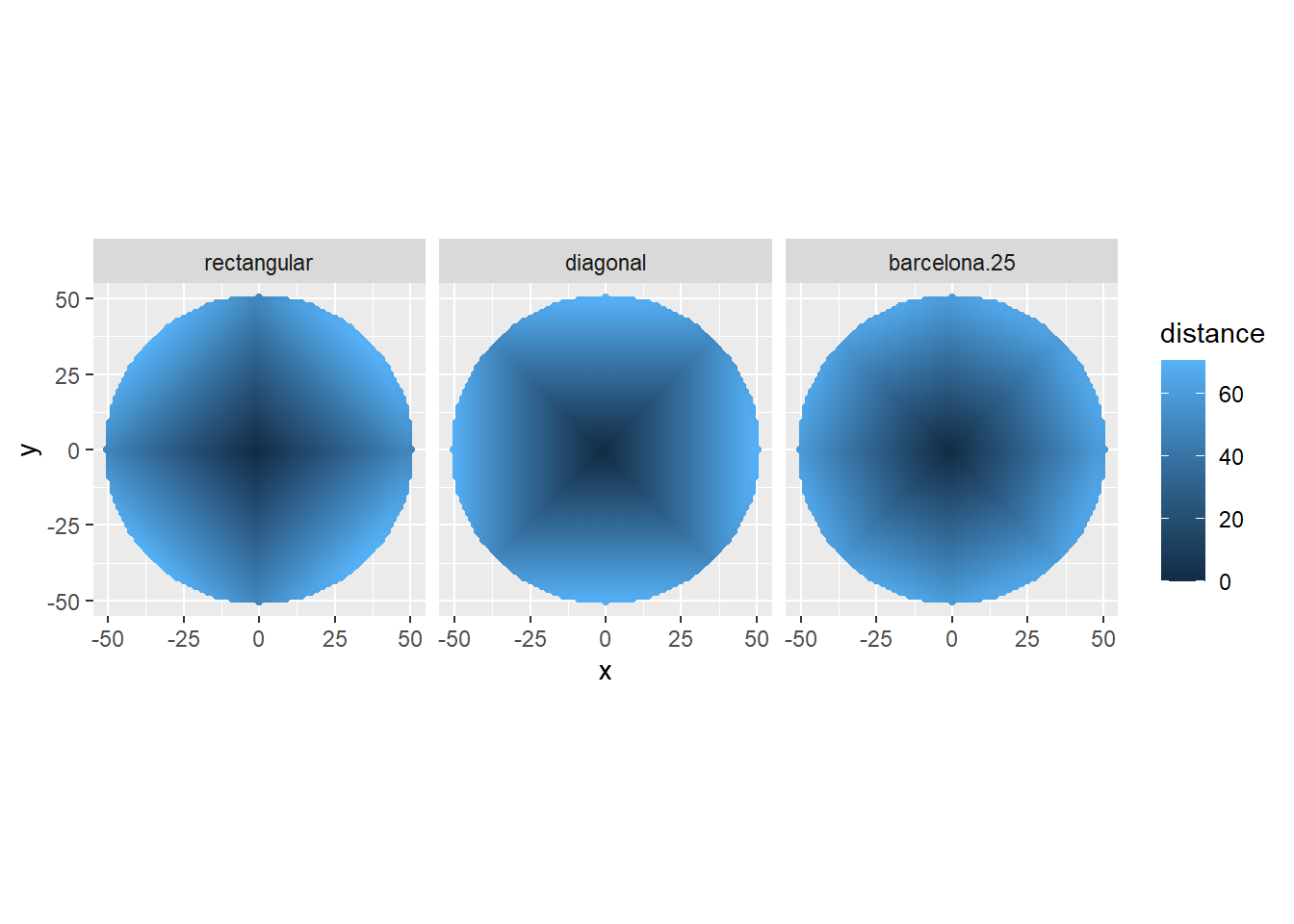
This suggests that if the city were square shaped (rather than a circle) that the transformed (diagonal and Barcelona) sidewalks would have greater than 50% of the residents with a shorter travel distance to the center of the city.
Transform grid, rotate first
add_transformation(
  m = matrix(c(0.5, 0.5,-0.5, 0.5), nrow = 2),
  seq_fun = seq_matrix_rotate_first) %>%
  animate_matrix()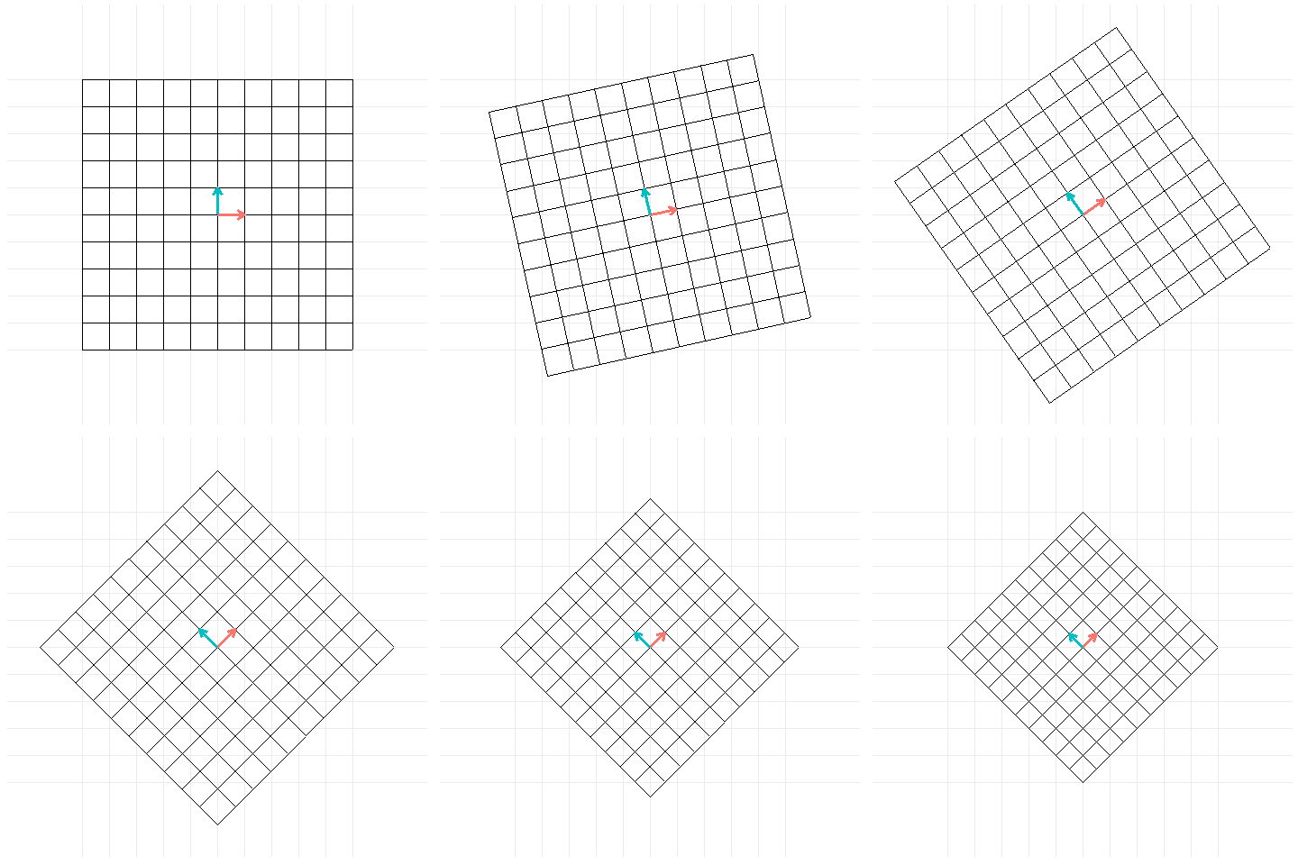
Transform city, pretty
start_grid <- animatrixr::construct_grid(-8:8, -8:8) %>%
  mutate(index = row_number(),
         time = 1L)

end_grid <- animatrixr::transform_segment(start_grid,  m = matrix(c(0.5, 0.5,-0.5, 0.5), nrow = 2)) %>%
  mutate(time = 2L)

house_points <- crossing(x = -3:3, y = -3:3) %>%
  mutate(symbol = emo::ji("house"))

city_hall <- tibble(x = 0, y = 0)

p_pretty <- bind_rows(start_grid, end_grid) %>%
  ggplot()+
  geom_segment(aes(x = x, y = y, xend = xend, yend = yend, group = index, colour = time))+
  geom_text(aes(x = x, y = y, label = symbol), data = house_points, size = 8)+
  geom_label(aes(x = x, y = y, label = "Riddler\nCity Hall"), data = city_hall, size = 8, color = "brown")+
  scale_colour_gradient(low = "black", high = "royalblue3")+
  scale_x_continuous(breaks = -3L:3L, minor_breaks = NULL)+
  scale_y_continuous(breaks = -3L:3L, minor_breaks = NULL)+
  coord_fixed(xlim = c(-3, 3), ylim = c(-3, 3))+
  theme_minimal()+
  theme(axis.text = element_blank(),
        axis.title = element_blank(),
        legend.position = "none",
        panel.border = element_rect(colour = "black", fill=NA, size=1))

p_pretty +
  gganimate::transition_states(time)
And wrote a couple preliminary posts on animating matrix transformations that can be found here and here↩︎
Is large enough to get a reasonable approximation for the answer.↩︎
I.e. straight line distance.↩︎
The Manhattan Length is just the shortest number of city blocks between points.↩︎
I highly recommend the Essence of Linear Algebra video series, particularly chapter 3 (on Matrix Transformations) and 13 (on Change of basis).↩︎
In R, you can use the
solve()function to give you the inverse of a matrix.↩︎We have already done most of the computations we’ll need and can follow similar steps to those taken in the Riddler Express solution.↩︎
I.e. length of an individual city block, or in this case, component of a city block.↩︎
In the diagram below, we will actually have it be a function of one-half of the inverse of the proportion – this is because there are two diagonals adjoining each horizontal component.↩︎
This can also be thought of as the diagonal and the horizontal side lengths can be thought of as a function of the side-length, x, of a triangle created by a diagonal.↩︎
Note that if we were to set x = 0, the distance from each location would be equivalent to the distances in our starting (horizontal) grid, and if we set x = 0.5, the distances would be equal to those in our transformed (diagonal) grid.↩︎
Note that we are not taking into account the tiny differences that emerge regarding starting location for each resident (i.e. which point within a Barcelona square should they start). If we make the grid arbitrarily large, these differences become inconsequential – hence we can ignore them.↩︎
The origin of our coordinate systems.↩︎