TLDR: In classification problems, under and over sampling1 techniques shift the distribution of predicted probabilities towards the minority class. If your problem requires accurate probabilities you will need to adjust your predictions in some way during post-processing (or at another step) to account for this2.
People new to predictive modeling may rush into using sampling procedures without understanding what these procedures are doing. They then sometimes get confused when their predictions appear way off (from those that would be expected according to the base rates in their data). I decided to write this vignette to briefly walk through an example of the implications of under or over sampling procedures on the base rates of predictions3.
My examples will appear obvious to individuals with experience in predictive modeling with imbalanced classes. The code is pulled largely from a few emails I sent in early to mid 20184 to individuals new to data science. Like my other posts, you can view the source code on github.
Note that this post is not about what resampling procedures are or why you might want to them5, it is meant only to demonstrate that such procedures change the base rates of your predictions (unless adjusted for).
The proportion of TRUE to FALSE cases of the target in binary classification problems largely determines the base rate of the predictions produced by the model. Therefore if you use sampling techniques that change this proportion (e.g. to go from 5-95 to 50-50 TRUE-FALSE ratios) there is a good chance you will want to rescale / calibrate6 your predictions before using them in the wild (if you care about things other than simply ranking your observations7).
library(tidyverse)
library(modelr)
library(ggplot2)
library(gridExtra)
library(purrr)

theme_set(theme_bw())
Create Data
Generate classification data with substantial class imbalance8.
# convert log odds to probability
convert_lodds <- function(log_odds) exp(log_odds) / (1 + exp(log_odds))

set.seed(123)

minority_data <- tibble(rand_lodds = rnorm(1000, log(.03 / (1 - .03)), sd = 1),
       rand_probs = convert_lodds(rand_lodds)) %>%
  mutate(target = map(.x = rand_probs, ~rbernoulli(100, p = .x))) %>%
  unnest() %>%
  mutate(id = row_number())

# Change the name of the same of the variables to make the dataset more
# intuitive to follow.
example <- minority_data %>%
  select(id, target, feature = rand_lodds)
In this dataset we have a class imbalance where our target is composed of ~5% positive (TRUE) cases and ~95% negative (FALSE) cases.
example %>%
  count(target) %>%
  mutate(proportion = round(n / sum(n), 3)) %>%
knitr::kable()| target | n | proportion |
|---|---|---|
| FALSE | 95409 | 0.954 |
| TRUE | 4591 | 0.046 |
Make 80-20 train - test split9.
set.seed(123)
train <- example %>%
  sample_frac(0.80)

test <- example %>%
  anti_join(train, by = "id")
Association of ‘feature’ and ‘target’
We have one important input to our model named feature10.
train %>%
  ggplot(aes(feature, fill = target))+
  geom_histogram()+
  labs(title = "Distribution of values of 'feature'",
       subtitle = "Greater values of 'feature' associate with higher likelihood 'target' = TRUE")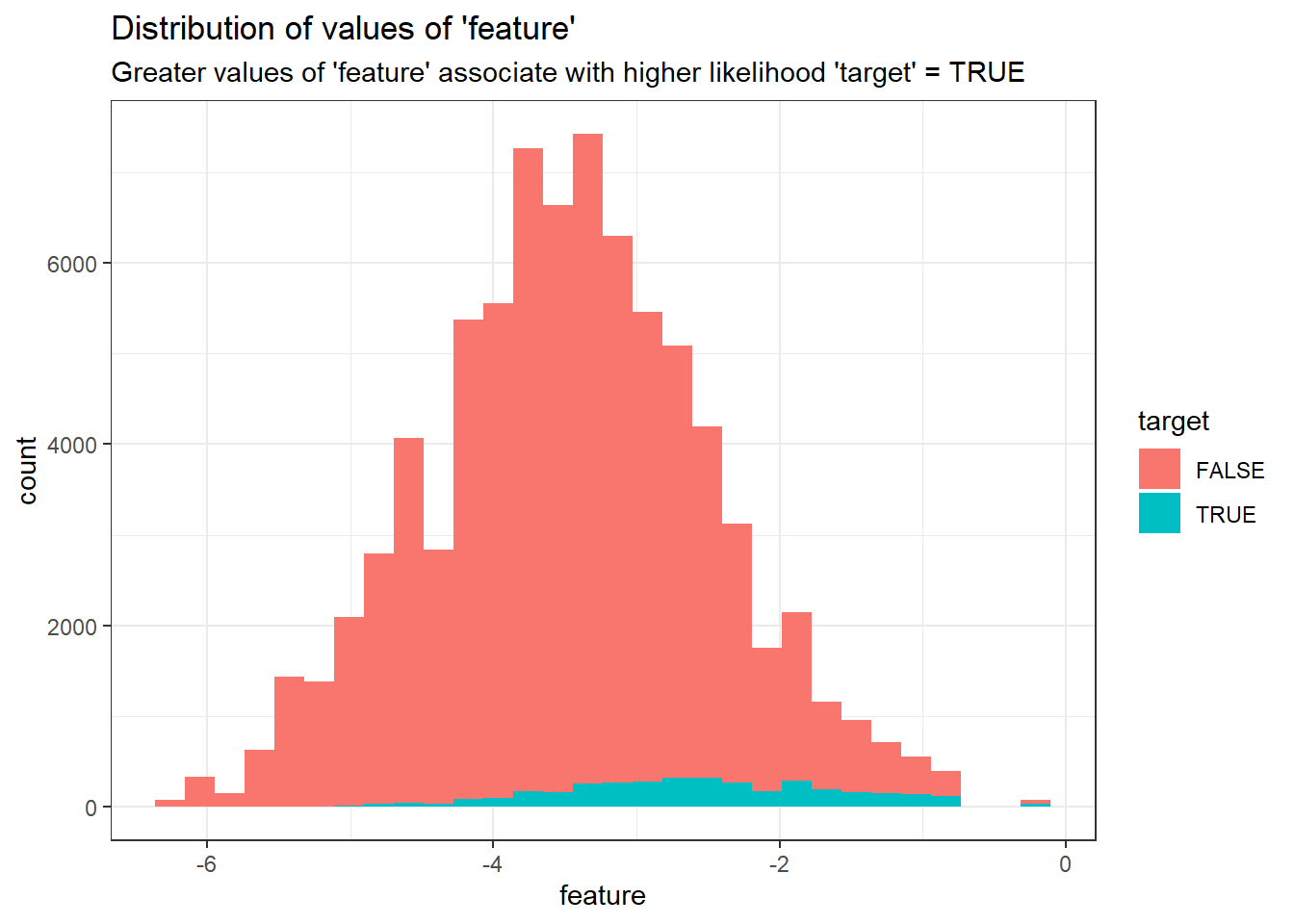
Resample
Make a new sample train_downsamp that keeps all positive cases in the training set and an equal number of randomly sampled negative cases so that the split is no longer 5-95 but becomes 50-50.
minority_class_size <- sum(train$target)

set.seed(1234)

train_downsamp <- train %>%
  group_by(target) %>%
  sample_n(minority_class_size) %>%
  ungroup()
See below for what the distribution of feature looks like in the down-sampled dataset.
train_downsamp %>%
  ggplot(aes(feature, fill = target))+
  geom_histogram()+
  labs(title = "Distribution of values of 'feature' (down-sampled)",
       subtitle = "Greater values of 'feature' associate with higher likelihood 'target' = TRUE")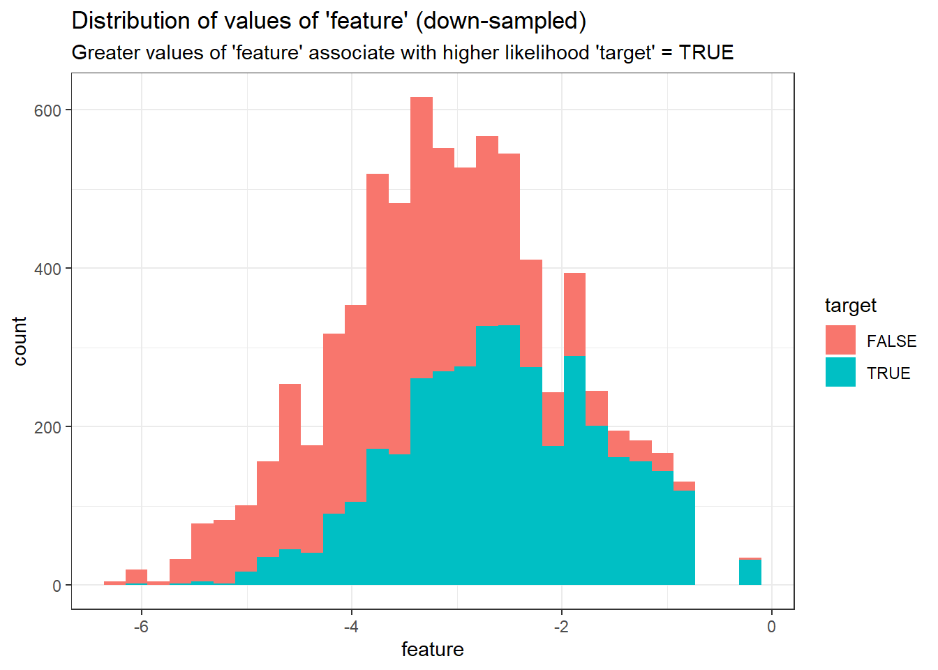
Build Models
Train a logistic regression model to predict positive cases for target based on feature using the training dataset without any changes in the sample (i.e. with the roughly 5-95 class imbalance).
mod_5_95 <- glm(target ~ feature, family = binomial("logit"), data = train)Train a model with the down-sampled (i.e. 50-50) dataset.
mod_50_50 <- glm(target ~ feature, family = binomial("logit"), data = train_downsamp)Add the predictions from each of these models11 onto our test set (and convert log-odd predictions to probabilities).
test_with_preds <- test %>%
  gather_predictions(mod_5_95, mod_50_50) %>%
  mutate(pred_prob = convert_lodds(pred))
Visualize distributions of predicted probability of the positive and negative cases for each model.
test_with_preds %>%
  ggplot(aes(x = pred_prob, fill = target))+
  geom_histogram()+
  facet_wrap(~model, ncol = 1)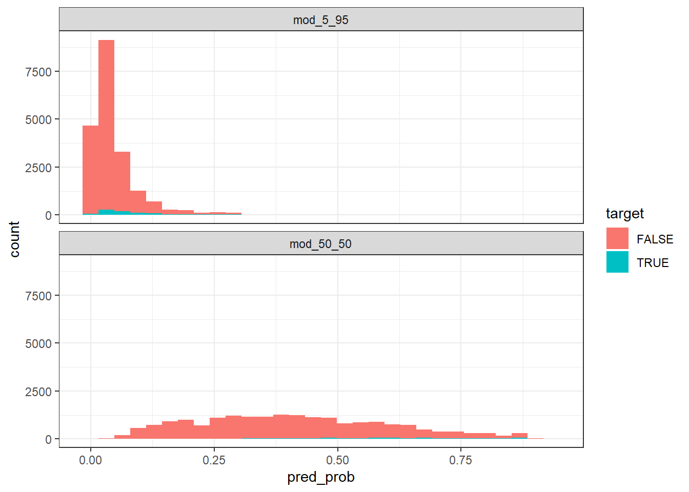
The predicted probabilities for the model built with the down-sampled 50-50 dataset are much higher than those built with the original 5-95 dataset. For example, let’s look at the predictions between these models for a particular observation:
test_with_preds %>%
  filter(id == 1828) %>%
  arrange(id) %>%
  select(-pred) %>%
knitr::kable(digits = 2)| model | id | target | feature | pred_prob |
|---|---|---|---|---|
| mod_5_95 | 1828 | FALSE | -2.77 | 0.06 |
| mod_50_50 | 1828 | FALSE | -2.77 | 0.56 |
This shows that when feature is equal to -2.77, the model built without undersampling produces a prediction of 6% whereas the model built from the undersampled data would predict 56%. The former can be thought of as the predicted probability of the event whereas the latter would first need to be rescaled.
If picking a decision threshold for the predictions, the model built from the undersampled dataset would have far more predictions of TRUE compared to the rate of TRUEs from the model built from the original training dataset12.
Rescale Predictions to Predicted Probabilities
Isotonic Regression13 or Platt scaling14 could be used. Such methods are used to calibrate outputted predictions and ensure they align with actual probabilities. Recalibration techniques are typically used when you have models that may not output well-calibrated probabilities15. However these methods can also be used to rescale your outputs (as in this case). (In the case of linear models, there are also simpler approaches available16.)
mod_50_50_rescaled_calibrated <- train %>%
  add_predictions(mod_50_50) %>%
  glm(target ~ pred, family = binomial("logit"), data = .)
test_with_preds_adjusted <- test %>%
spread_predictions(mod_5_95, mod_50_50) %>%
rename(pred = mod_50_50) %>%
spread_predictions(mod_50_50_rescaled_calibrated) %>%
select(-pred) %>%
gather(mod_5_95, mod_50_50_rescaled_calibrated, key = "model", value = "pred") %>%
mutate(pred_prob = convert_lodds(pred))
test_with_preds_adjusted %>%
ggplot(aes(x = pred_prob, fill = target))+
geom_histogram()+
facet_wrap(~model, ncol = 1)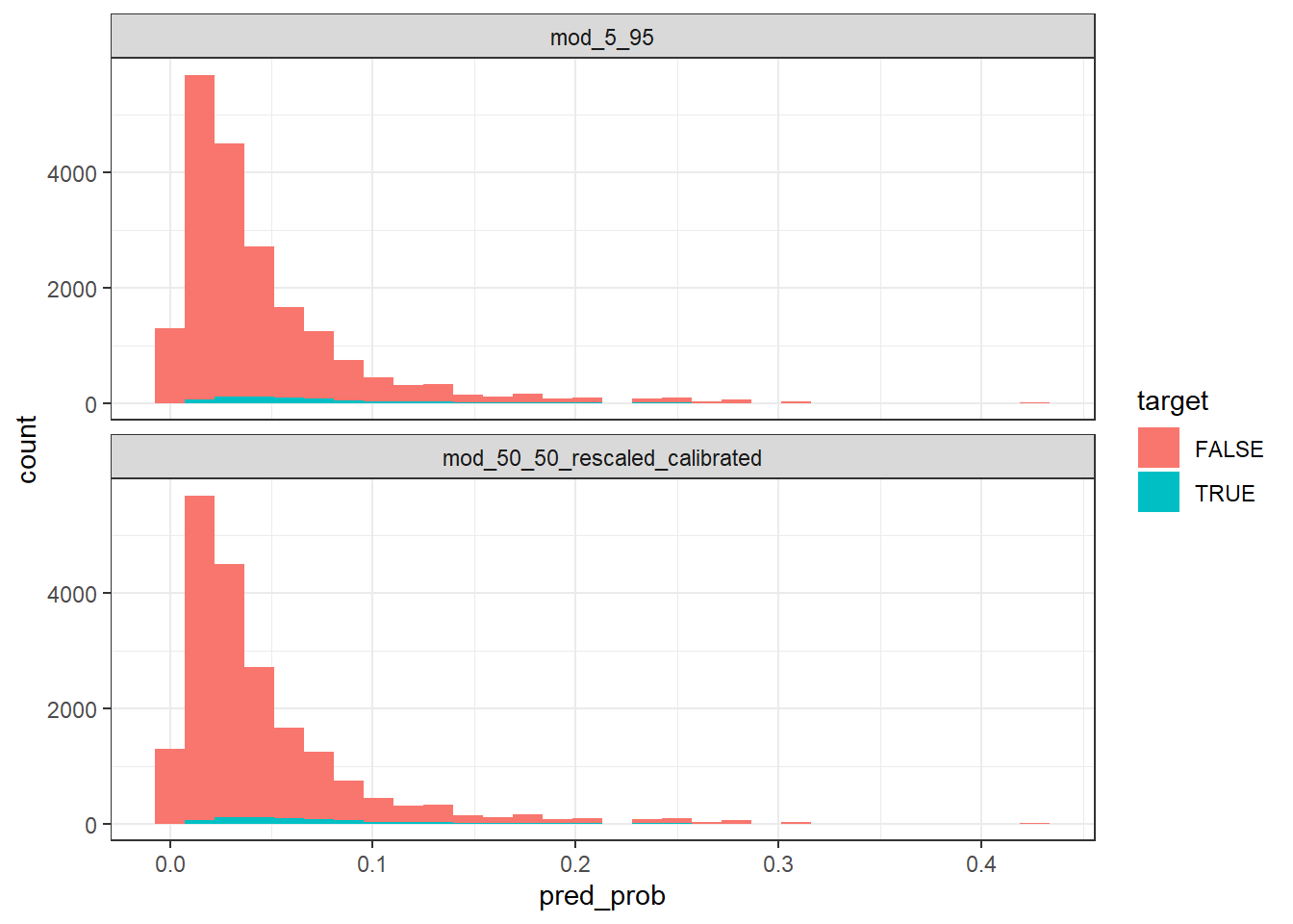
Now that the predictions have been calibrated according to their underlying base rate, you can see the distributions of the predictions between the models are essentially the same.
Appendix
Density Plots
Rebuilding plots but using density distributions by class (rather than histograms based on counts).
test_with_preds %>%
  ggplot(aes(x = pred_prob, fill = target))+
  geom_density(alpha = 0.3)+
  facet_wrap(~model, ncol = 1)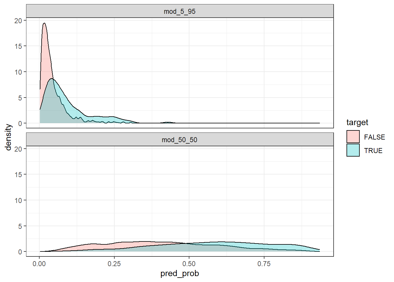
test_with_preds_adjusted %>%
  ggplot(aes(x = pred_prob, fill = target))+
  geom_density(alpha = 0.3)+
  facet_wrap(~model, ncol = 1)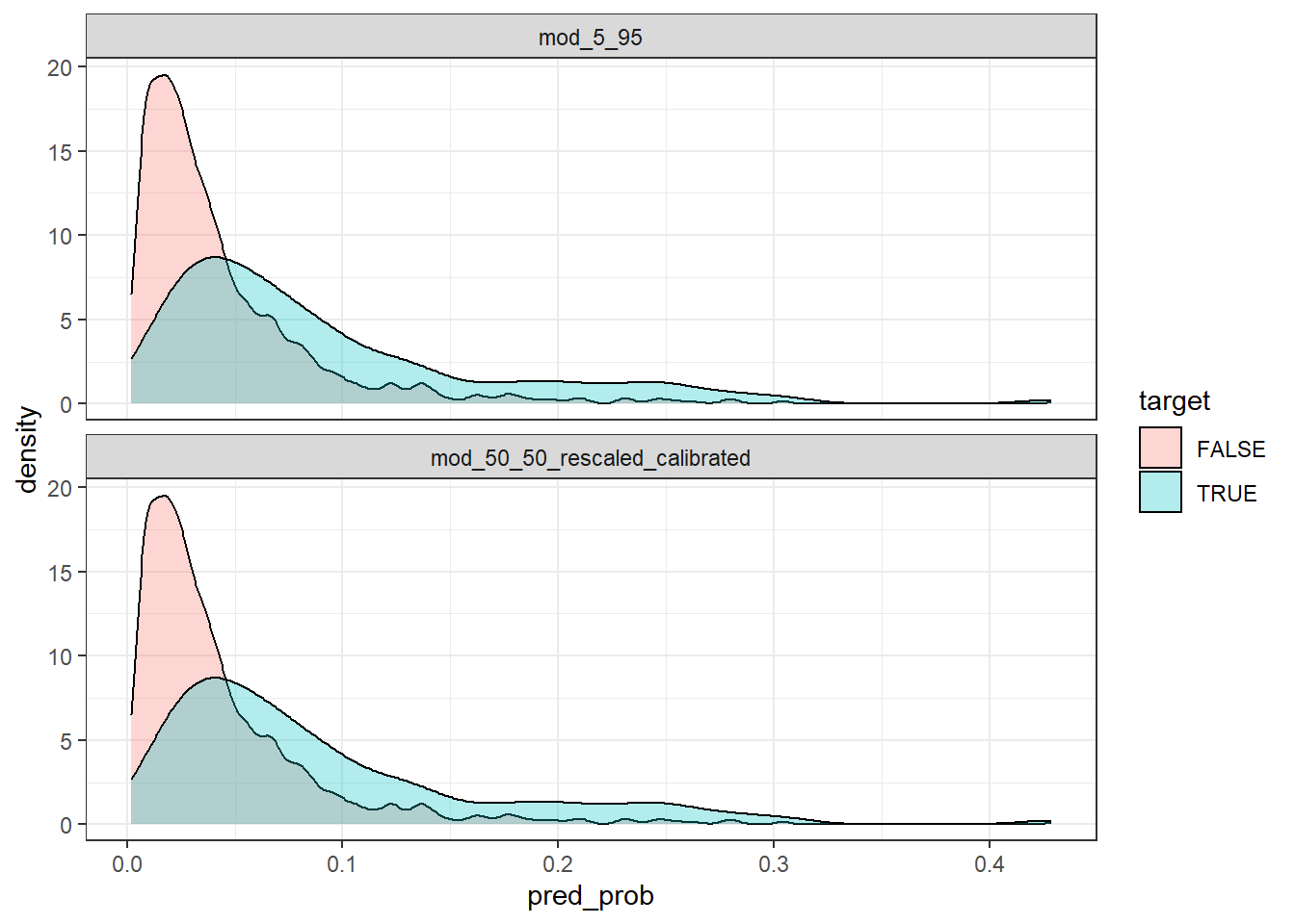
Lift Plot
test_with_preds_adjusted %>%
  mutate(target = factor(target, c("TRUE", "FALSE"))) %>%
  filter(model == "mod_5_95") %>%
  yardstick::lift_curve(target, pred) %>%
  autoplot()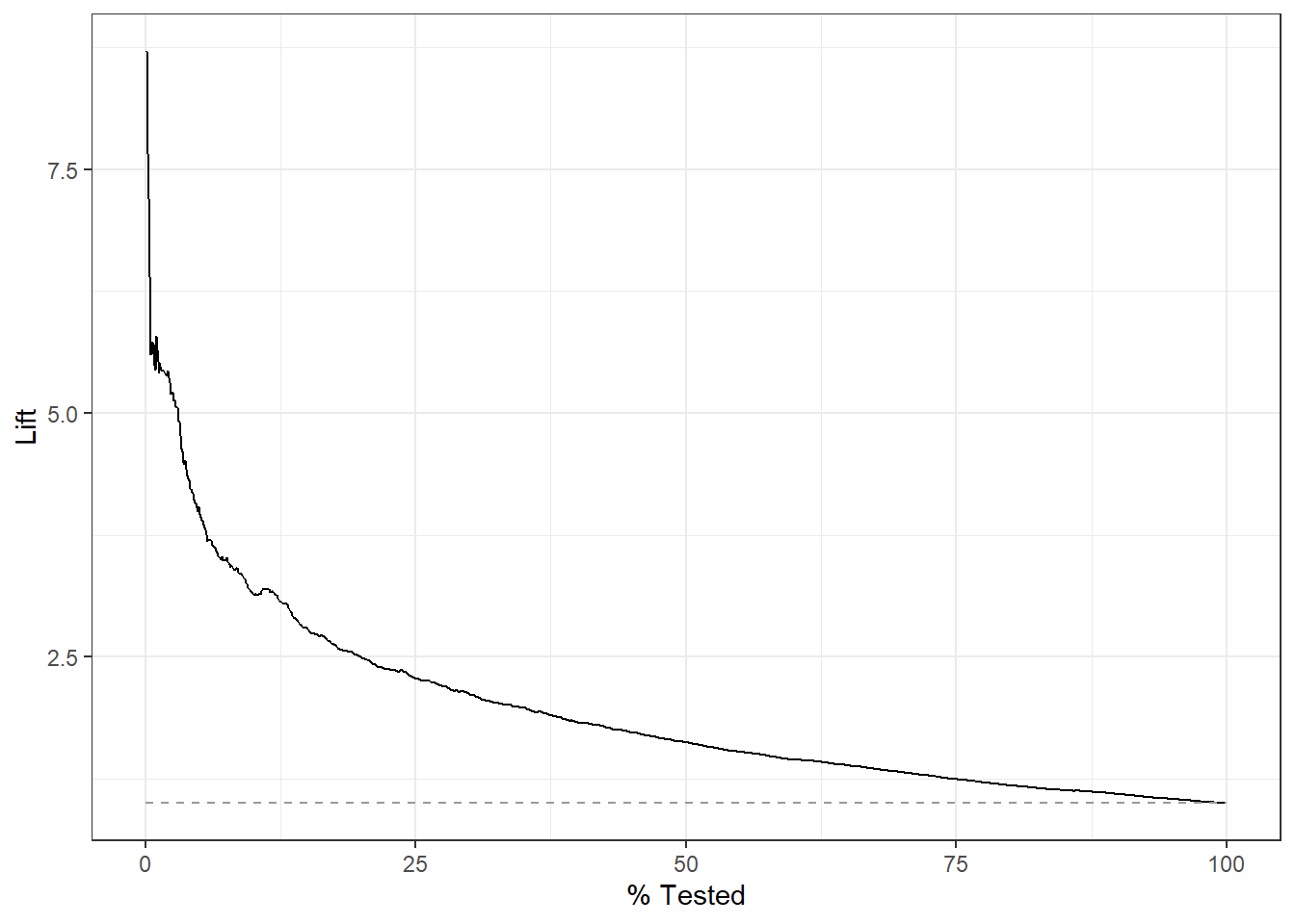
Comparing Scaling Methods
Added after publishing
Thanks to Andrew Wheeler for his helpful disqus comment referencing another method for rescaling which prompted me to create a quick gist comparing platt scaling against using an offset/adjustment approach for rescaling.
In the title I just mention Undersamping for brevities sake. Upsampling and downsampling are synonyms you may hear as well↩︎
I expect the audience for this post may be rather limited.↩︎
I wrote this example After having conversations related to this a few times (and participants not grasping points that would become clear with demonstration).↩︎
before I started using tidymodels↩︎
or any of a myriad of topics related to this.↩︎
There are often pretty easy built-in ways to accommodate this.↩︎
There are also other reasons you may not want to rescale your predictions… but in many cases you will want to.↩︎
Could have been more precise here…↩︎
no need for validation for this example↩︎
The higher incidence of TRUE values in the target at higher scores demonstrates the features predictive value.↩︎
One built with 5-95 split the other with a downsampled 50-50 split.↩︎
Of course you could just use different decision thresholds for the predictions as well.↩︎
Decision tree based approach↩︎
Logistic regression based approach↩︎
E.g. when using Support Vector Machines↩︎
In this case we are starting with a linear model hence we could also have just changed the intercept value to get the same affect. Rescaling methods act on the predictions rather than the model parameters. Hence these scaling methods have the advantage of being generalizable as they are agnostic to model type.↩︎