Weighting in predictive modeling may take multiple forms and occur at different steps in the model building process.
- When selecting observations to be used in model training
- During model training
- After model training, during model evaluation
The focus of this post is on the last stage1. I will describe two types of weighting that can be applied in late stage model evaluation:
Specifically with the aim of identifying ideal cut-points for making class predictions.
(See Weights of Observations During and Prior to Modeling in the Appendix for a brief discussion on forms of weighting applied at other steps in predictive modeling.)
Model Performance Metrics
Most common metrics used in classification problems – e.g. accuracy, precision, recall/sensitivity, specificity, Area Under the ROC curve2 (AUC) or Precision-Recall curve – come down to the relationship between the true positives (TP), true negatives (TN), false positives (FP), and false negatives (FN) at a particular decision threshold3 or across all thresholds4. Initial model evaluation and selection should generally start by reviewing metrics that capture general performance across all thresholds. Max Kuhn and Kjell Johnson explain this in their book Feature Engineering and Selection…:
“During the initial phase of model building, a good strategy for data sets with two classes is to focus on the AUC statistics from these curves instead of metrics based on hard class predictions. Once a reasonable model is found, the ROC or precision-recall curves can be carefully examined to find a reasonable cutoff for the data and then qualitative prediction metrics can be used.” - 3.2.2 Classification Metrics
Once a performant model has been selected, the analyst can then identify an ideal decision threshold/cut-point/cutoff for making class predictions. In this post I will largely be skipping this initial phase in model building. Instead I will focus on methods for identifying optimal cutoffs. In particular, I will use weights on predictions and outcomes (on a hold-out-dataset) to determine which decision thresholds would maximize expected value for a selected model5.
Every Cut-Point Has an Associated Confusion Matrix
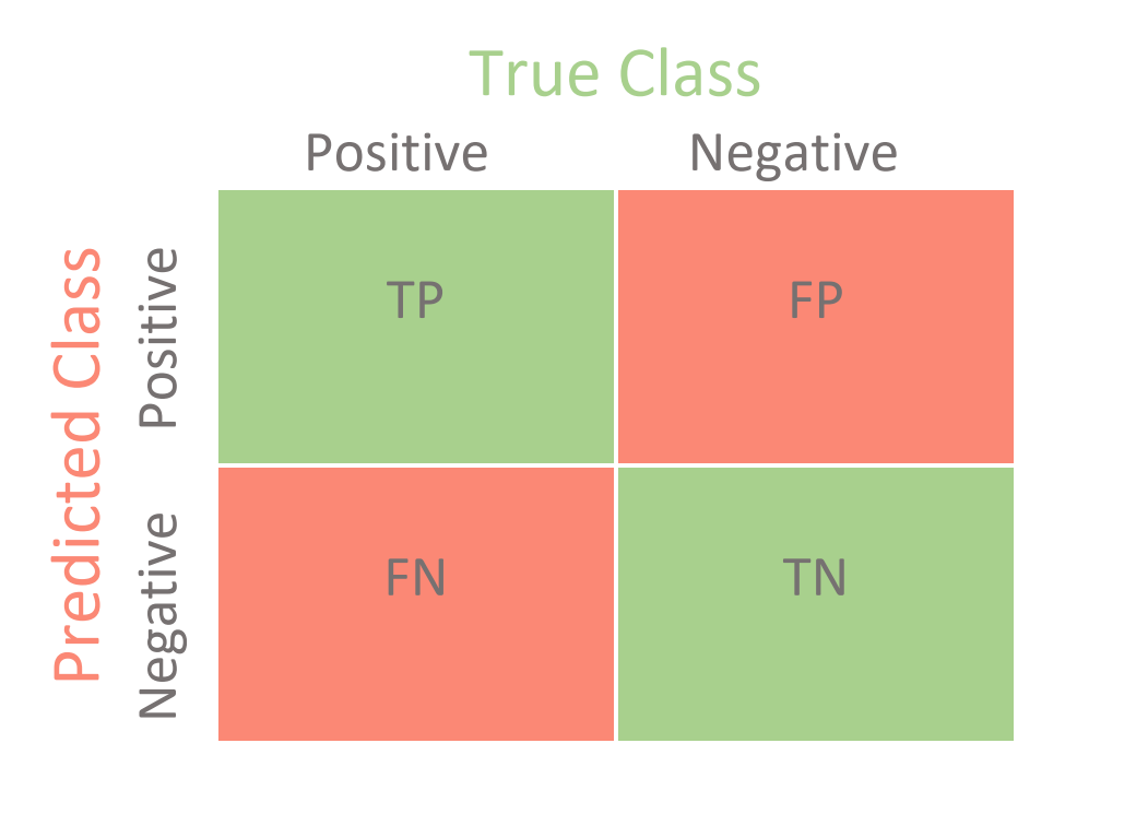
The frequency of classification outcomes (TP, TN, FP, FN) at a specific decision threshold are often represented by a confusion matrix.
Each cell of a confusion matrix may represent a more or less valuable outcome depending on the particular problem. In the case of giving out loans, a false positive may be more costly than a false negative6 while in problems concerning security threats the reverse may be true7. When you have a sense of the value associated with the classification outcomes, you can use this information to weight the confusion matrices, calculate the expected value of each, identify which maximizes expected value and select the associated decision threshold for use when deploying your model.
Note that weighting applied in the evaluation stage (as discussed throughout this post) often relies on the predicted probabilities of your model being accurate (and not just ranked correctly)8.
Lending Data Example
Lending Club data is used for examples throughout this post. I will be predicting the binary target Class, which defines whether loans are in good or bad standing (i.e. whether the recipient is or is not in default on their loan).
Load packages, set theme, load data:
library(parsnip)
library(probably)
library(rsample)
library(modeldata)
library(yardstick)
library(tidyverse)

theme_set(theme_minimal())

data("lending_club")
Starter Code
This section provides a brief example of building a model and calculating a confusion matrix at a particular decision threshold. Most of the code in this section is copied from a vignette for the probably9 package and will serve as starter code for my examples. I provide brief descriptions of the code chunks but recommend reading the source for explanations on the steps.
(If you are familiar with tidymodels and modeling in classification problems you might skip to Weighting by Classification Outcomes.)
Minor transformations and select relevant columns:
lending_club <- lending_club %>%
  mutate(Class = relevel(Class, "good")) %>%
  select(Class, annual_inc, verification_status, sub_grade, funded_amnt)
Training / Testing split:
set.seed(123)
split <- rsample::initial_split(lending_club, prop = 0.75)

lending_train <- rsample::training(split)
lending_test  <- rsample::testing(split)
Specify and build model:
logi_reg <- logistic_reg()
logi_reg_glm <- logi_reg %>%
  set_engine("glm")

logi_reg_fit <- fit(
  logi_reg_glm,
  formula = Class ~ annual_inc + verification_status + sub_grade,
  data = lending_train
)
Add predictions to test set:
predictions <- logi_reg_fit %>%
  predict(new_data = lending_test, type = "prob")

lending_test_pred <- bind_cols(predictions, lending_test)
Use probably::make_two_class_pred() to make hard predictions at a threshold of 0.50:
hard_pred_0.5 <- lending_test_pred %>%
  mutate(.pred = probably::make_two_class_pred(.pred_good,
                                               levels(Class),
                                               threshold = 0.5) %>%
           as.factor(c("good", "bad"))
         ) %>%
  select(Class, contains(".pred"))
After we’ve made class predictions we can make a confusion matrix10. Use yardstick::conf_mat() to get a confusion matrix for the class predictions:
conf_mat_0.5 <- yardstick::conf_mat(hard_pred_0.5, Class, .pred)

conf_mat_0.5 %>% autoplot(type = "heatmap")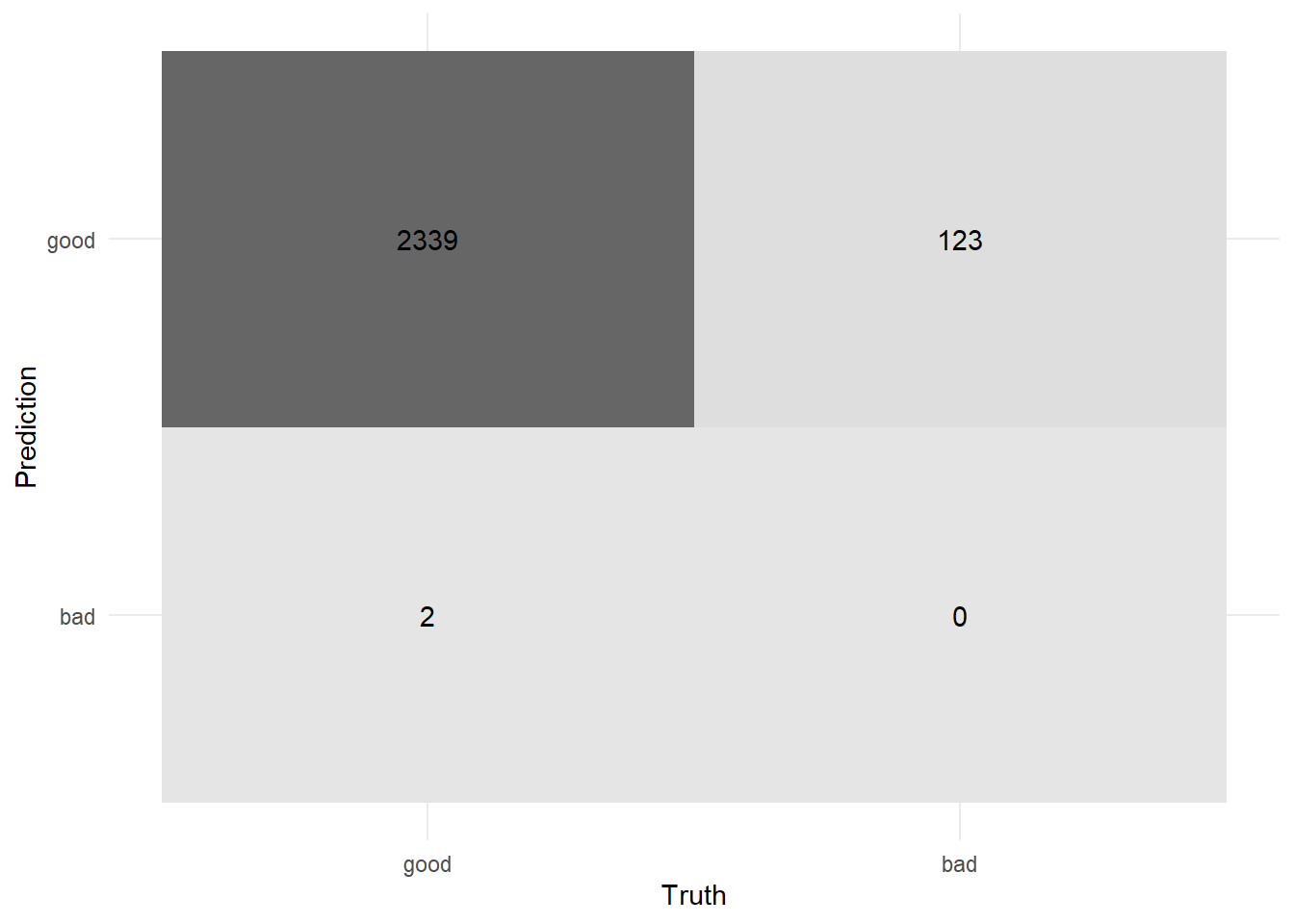
We could also call summary(conf_mat_0.5) to calculate common metrics at this decision threshold.
Custom function:
I will load in a function conf_mat_weighted() that works similarly to yardsitck::conf_mat() but can handle observation weights (which will come into play in Weighting by Observations).
# source conf_mat_weighted() which is similar to yardstick::conf_mat() but also
# has the possibility of handling a weights column
devtools::source_gist("https://gist.github.com/brshallo/37d524b82541c2f8540eab39f991830a")
Weighting by Classification Outcomes
For the purposes of this post I will bypass common steps in model evaluation and selection and go straight to using weighting techniques to identify appropriate decision thresholds for a selected model11.
For our loan problem we will use the following weighting scheme for our potential classification outcomes:
- TP: 0.14 (predict a loan is good when it is indeed good)
- FP: 3.10 (predict a loan is good when it is actually bad)
- TN: 0.02 (predict a loan is bad when it is indeed bad)
- FN: 0.06 (predict a loan is bad when it is actually good)
\[ Weights = \left(\begin{array}{cc} 0.14 & 3.10\\0.06 & 0.02 \end{array}\right)\]
There may be asymmetries in business processes associated with the ‘actual’ and the ‘predicted’ states that might explain differences in the value associated with each cell in the confusion matrix12.
I put the classification outcome weights into a matrix13.
outcome_weights <- matrix(
          c(0.14, 3.1,
          0.06, 0.02),
          nrow = 2,
          byrow = TRUE
)
Next I apply these weights to the cells of the confusion matrix.
weight_cells <- function(confusion_matrix, weights = matrix(rep(1, 4), nrow = 2)){

  confusion_matrix_output <- confusion_matrix
  confusion_matrix_output$table <- confusion_matrix$table * weights
  confusion_matrix_output
}

conf_mat_0.5_weighted <- weight_cells(conf_mat_0.5, outcome_weights)

conf_mat_0.5_weighted %>% autoplot(type = "heatmap")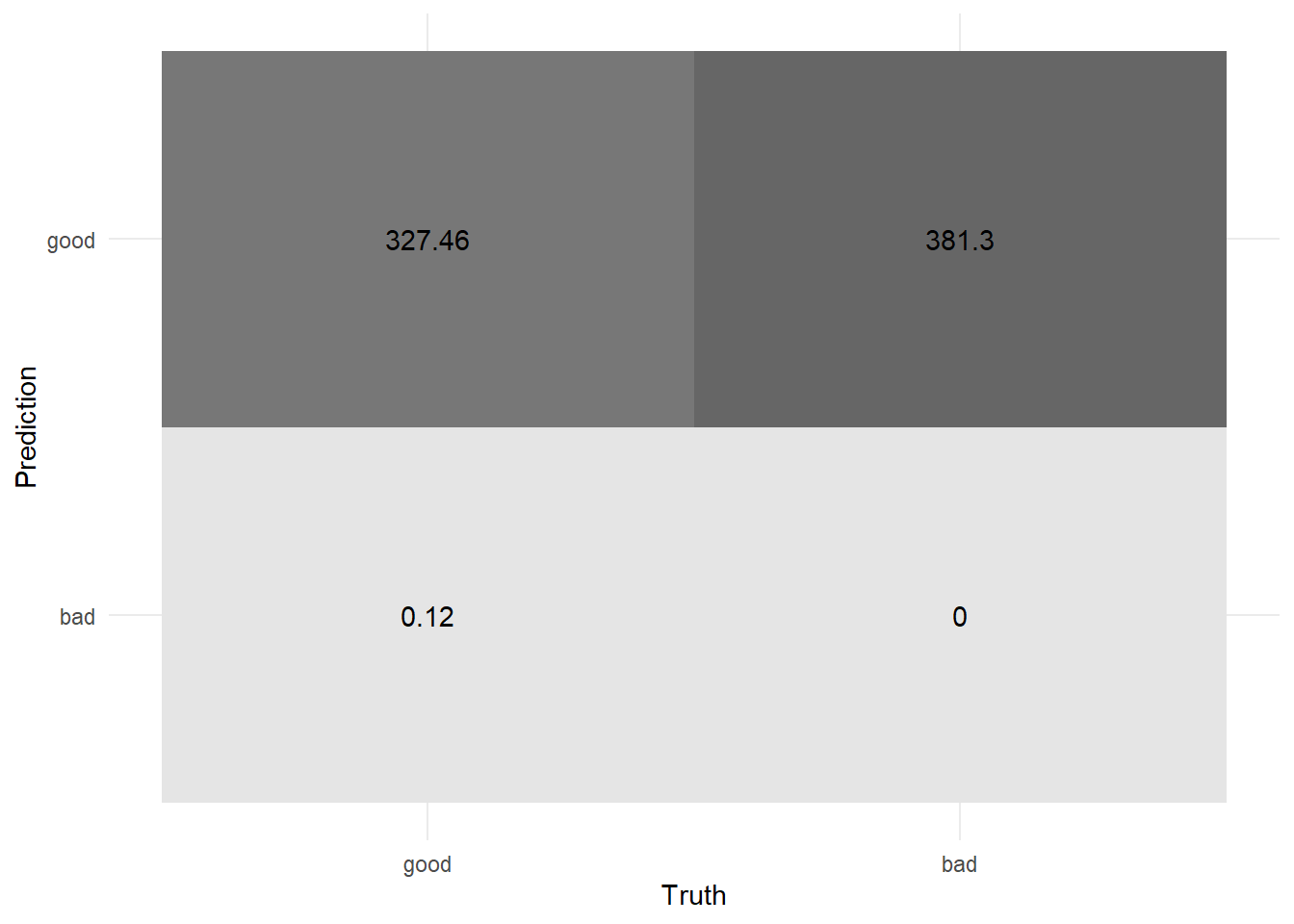
Notice how different these values are from those calculated without weighting (shown in Starter Code).
An earlier version of this post included a variety of other performance metrics calculated after weighting by classification outcomes. See Weighted Classification Metrics in the Appendix for a discussion on why these were removed from the body of the post.
Assuming diagonal (correctly predicted) elements represent a gain14 and off-diagonal elements a loss15, I will calculate the total value at the 0.50 decision threshold (by taking the difference of the aggregated gains and losses)16.
sum( (conf_mat_0.5$table * outcome_weights) * matrix(c(1,-1,-1, 1), byrow = TRUE, ncol = 2) )## [1] -53.96At a prediction threshold for accepting loans of 0.50, our expected value would be negative.
Metrics Across Decision Thresholds
We do not want to see performance at just the individual cut-point of 0.50 but across the range of possible decision thresholds17.
I wrote a function conf_mat_threshold() that first creates hard predictions based on a threshold and then creates the associated confusion matrix at that threshold.
#' Confusion Matrix at Threshold
#'
#' @param df dataframe containing a column `.pred_good`.
#' @param threshold A value between 0 and 1.
#' @param wt A column that gets passed into `conf_mat_weighted()` if also wanting to give observation weights (default is NULL).
#'
#' @return a confusion matrix
conf_mat_threshold <- function(df = lending_test_pred,
                               threshold = 0.5,
                               ...){
  hard_pred <- df %>%
    mutate(.pred = probably::make_two_class_pred(.pred_good,
                                                 levels(Class),
                                                 threshold = threshold) %>%
             as.factor(c("good", "bad"))
           )

  conf_mat_weighted(hard_pred, Class, .pred, ...)
}
I will map the conf_mat_threshold()18 function across all meaningful cut-points in the dataset (creating confusion matrices at each). Next I will use weight_cells() to weight the resulting confusion matrices by the outcome weights.
# get all unique predictions that differ by at least 0.001
thresholds_unique_df <- tibble(threshold = c(0, unique(lending_test_pred$.pred_good), 1)) %>%
  arrange(threshold) %>%
  mutate(diff_prev = abs(lag(threshold) - threshold),
         diff_prev_small = ifelse((diff_prev) <= 0.001, TRUE,FALSE),
         diff_prev_small = ifelse(is.na(diff_prev_small), FALSE, diff_prev_small)) %>%
  filter(!diff_prev_small) %>%
  select(threshold)
# compute confusion matrices and weighted confusion matrices
conf_mats_df <- thresholds_unique_df %>%
mutate(conf_mat = map(threshold, conf_mat_threshold, df = lending_test_pred)) %>%
mutate(conf_mat_weighted = map(conf_mat, weight_cells, weights = outcome_weights))I then use total_value() to calculate the expected value at each threshold and plot these across cut-points:
total_value <- function(weighted_conf_matrix){
  sum(weighted_conf_matrix * matrix(c(1, -1, -1, 1), byrow = TRUE, ncol = 2))
}

conf_mats_value <- conf_mats_df %>%
  arrange(desc(threshold)) %>%
  mutate(value = map_dbl(conf_mat_weighted, ~total_value(.x$table)))

conf_mats_value %>%
  ggplot(aes(x = threshold, y = value))+
  geom_line()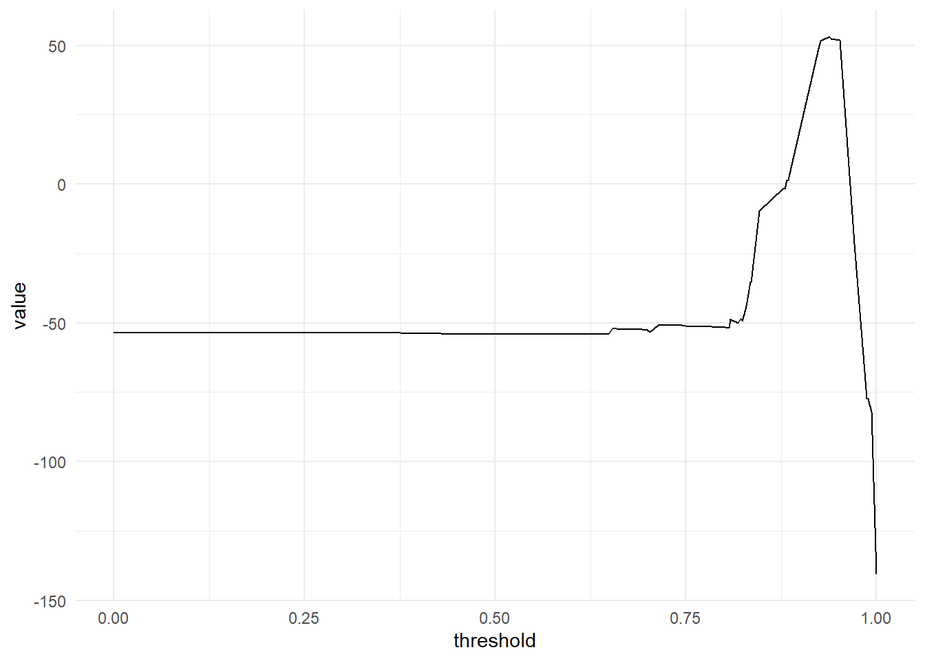
This suggests the greatest value occurs when using a threshold between 0.93 and 0.9619. Value suffers a steep drop-off at either end of this range (quickly turning negative). For comparison, an unweighted metric would have suggested predicting “Bad” loans for everything20.
Below is the confusion matrix and the weighted confusion matrix at the ideal cut-point of ~0.94 (the former corresponds with raw observation counts and the latter with the value of those counts):
cfm1 <- conf_mats_value %>%
  arrange(desc(value)) %>%
  pluck("conf_mat", 1) %>%
  autoplot(type = "heatmap")+
  coord_fixed()+
  labs(title = "Confusion Matrix",
       subtitle = "Threshold: 0.94")

cfm2 <- conf_mats_value %>%
  arrange(desc(value)) %>%
  pluck("conf_mat_weighted", 1) %>%
  autoplot(type = "heatmap")+
  coord_fixed()+
  labs(title = "Value Weighted Confusion Matrix",
       subtitle = "Threshold: 0.94")

library(patchwork)

cfm1 + cfm2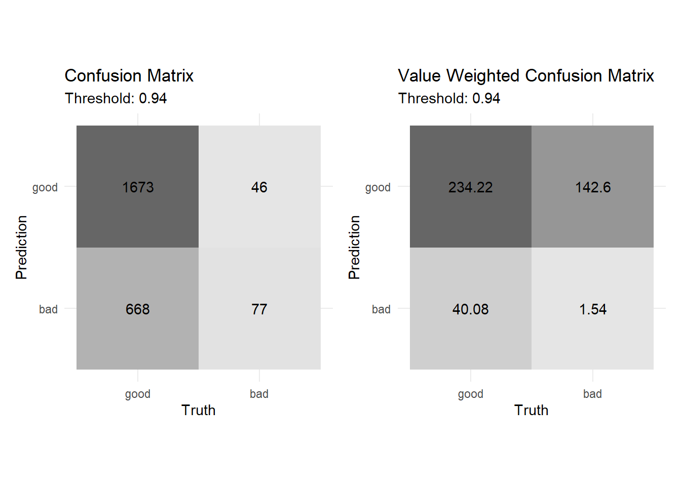
Weighting by Observations
In the prior section, we used weights to represent the value of classification outcomes. What if we want to account for the value of a specific loan (since higher loan amounts might amplify possible risks)? In this section I will apply the same steps as above but will first weight individual observations21 by the funded_amnt column22.
My function conf_mat_weighted() (sourced from gist previously) can handle a value for observation weights. Hence, we will follow the same steps as in Weighting by Classification Outcomes except also supplying wt = funded_amnt.
# get confusion matrices and weighted confusion matrices
conf_mats_df_obs_weights <- thresholds_unique_df %>%
  mutate(conf_mat = map(threshold,
                        conf_mat_threshold,
                        df = lending_test_pred,
                        # funded_amnt provides observation weights
                        wt = funded_amnt)) %>%
  mutate(conf_mat_weighted = map(conf_mat, weight_cells, weights = outcome_weights)) %>%
  mutate(across(contains("conf"), list(metrics = ~map(.x, summary))))
The range of cut-points that maximizes ‘value’ appears similar to that shown in the previous section (when not weighting observations by funded_amnt):
conf_mats_df_obs_weights %>%
  arrange(desc(threshold)) %>%
  mutate(value = map_dbl(conf_mat_weighted, ~total_value(.x$table))) %>%
  discard(is.list) %>%
  ggplot(aes(x = threshold, y = value))+
  geom_line()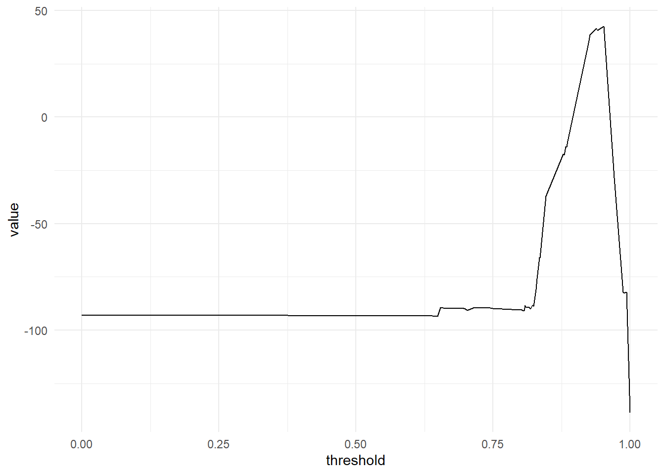
Closing note
Once you’ve developed a well-calibrated model, weighting by classification outcomes and observation weights can be helpful for identifying an optimal decision threshold that will maximize expected value when making class predictions.
Appendix
Weights of Observations During and Prior to Modeling and (maybe) Notes on Cost Sensitive Classification are the only sections people other than the author are likely to find interesting.
Other sections are primarily bookmarks on thought-processes related to earlier versions of this post. I was unsure about the appropriateness of calculating weighted classification metrics as well as which weighting scheme I wanted to use. See question on Cross Validated and sections Questions on Cost Sensitive Classification, Weighted Classification Metrics, and Arriving at Weights for questions I wrestled with while writing this post.
Weights of Observations During and Prior to Modeling
The body of the blog post is focused exclusively on weighting in model evaluation after model training. This section provides a brief overview of other types of weighting that can be used in modeling (as well as references for these topics).
Robert Moser has a helpful blog post, Fraud detection with cost sensitive machine learning, where he differentiates cost dependent classification (weighting after model building) from cost sensitive training (the practice of baking in the costs of classification outcomes23 into the objective function used during model training24). Some modeling algorithms may inherently weight observations differently. For example, in the regression context, Weighted Least Squares will adjust observations weights to reduce the impact of highly influential observations.
In other cases, weights are applied not in the model building step but immediately prior when setting the likelihood of an observation to be selected for training the model. For example, undersampling, oversampling or other sampling techniques are typically used in attempts to improve the performance of a model in predicting a minority class25 but can also be used as a means of changing the base rate associated with each class26. Some algorithms use biased resampling techniques directly in their model building procedures27. Similar in effect to over and under sampling the data, models may also handle weights according to the outcome class of the observation28.
Notes on Cost Sensitive Classification
Depending on your problem you might also use different approaches for weighting confusion matrices after model building. To account for differences in the value of classification outcomes you might weight items in the confusion matrix more heavily depending on what their actual condition is (e.g. TRUE outcomes are weighted higher than FALSE outcomes). You might also use a cost based approach to evaluate performance, whereby the diagonal elements on the confusion matrix (the correctly predicted items) have a cost of zero and all other cells are weighted according to their associated costs (see Questions on Cost Sensitive Classification for further discussion on these).
Some notes on implementations:
- The mlr package provides a helpful vignette (Cost-Sensitive Classification) that covers a variety of these and other approaches29.
- In python the costcla module provides documentation on how to approach many of these types of problems in python.
- Unfortunately, the
tidymodelssuite of packages does not yet have broad support for weights. There are some relevant open issues, e.g. #3 inyardstickdescribes approaches for cost sensitive metrics.
Weighted Classification Metrics
I posted a question to Cross Validated (CV) on Weighting common performance metrics by classification outcomes?. I also reached out to other analytics professionals relating my questions about these metrics. I ultimately came to the conclusion that many performance metrics weighted by classification outcomes are inappropriate (other than expected value) or not useful so kept the focus of this post on using weighted classification outcomes strictly for maximizing expected value and identifying ideal cut-points on an already selected model.
I also changed my weighting scheme though not such that any cells in the confusion matrix would be zeroed out30.
Weighted performance metrics on a confusion matrix at threshold of 0.5:
summary(conf_mat_0.5_weighted) %>%
knitr::kable(digits = 3)| .metric | .estimator | .estimate |
|---|---|---|
| accuracy | binary | 0.462 |
| kap | binary | 0.000 |
| sens | binary | 1.000 |
| spec | binary | 0.000 |
| ppv | binary | 0.462 |
| npv | binary | 0.000 |
| mcc | binary | -0.014 |
| j_index | binary | 0.000 |
| bal_accuracy | binary | 0.500 |
| detection_prevalence | binary | 1.000 |
| precision | binary | 0.462 |
| recall | binary | 1.000 |
| f_meas | binary | 0.632 |
Weighted performance metrics across decision thresholds:
conf_mats_df %>%
  mutate(across(contains("conf"), list(metrics = ~map(.x, summary)))) %>%
  unnest(conf_mat_weighted_metrics) %>%
  select(-contains("conf"), -.estimator) %>%
  filter(.metric != "sens") %>%
  ggplot(aes(x = threshold, y = .estimate))+
  geom_line()+
  facet_wrap(~.metric, scales = "free_y")+
  labs(title = "Weighted Performance Metrics")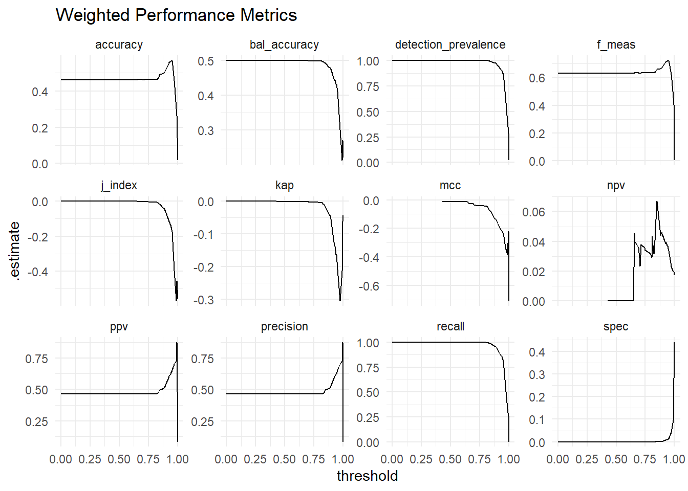
Interpretation of these metrics is unclear (as described on the CV issue mentioned above).
Questions on Cost Sensitive Classification
I was unsure on which type of weighting scheme I wanted to use for this post. This section walks through some of the questions I asked myself related to this.
Resources on cost based approaches to model evaluation of classification problems seemed to take a variety of different approaches. This left me with a few questions about what is appropriate and what is inappropriate.
Should the diagonal elements be zero?
Most of the examples I saw on cost-sensitive classification had their correctly predicted items (the diagonal of the confusion matrix) set to zero (assuming no or small costs associated with correctly predicted outcomes)31. There are some exceptions to this:
- Sowmya Vivek provides an example of this in her article Model performance & cost functions for classification models.
- Robert Moser’s post on Fraud detection with cost sensitive machine learning
These gave me some confidence that there isn’t a problem with having non-zero items on the diagonals.
Should off-diagonal elements be negated?
I did notice that Moser only used positive weighting whereas Vivek’s post had the weights sign negated depending on if it was on the diagonal or off-diagonal. I prefer Moser’s approach as I figure the signs could be negated when evaluating ‘value’ (which is the approach that I took32).
Do weighted classification metrics make sense?
When weighting a confusion matrix, does it also make sense to calculate other weighted metrics, e.g. weighted precision, recall, etc.? Does it make sense to look at these across decision thresholds33? The problem with the weighted versions of these metrics is that the possible number of observations could essentially change between decision cut-points because of observations slipping between higher or lower weighted classification outcomes. Does this present a mathematical challenge of some sort? Clearly if some cells are weighted to 0, some performance metrics may not make sense to calculate34.
I ended-up posting this question on cross validated: Weighting common performance metrics by classification outcomes?.
Arriving at Weights
I initially used a different set of weights:
\[ Weights = \left(\begin{array}{cc} 0.14 & 1.89\\1.86 & 0.11 \end{array}\right)\]
I think this approach was an example of thinking too hard and that the approach here is incorrect or at least unnecessary… I also ended-up using a different set of weights (that were just made-up).
Say there are three things that determine how value should be weighted across a confusion matrix:
- How value is spread across the actual dimension
- How value is spread across the predicted dimension
- How value is shared between the actual and predicted dimensions
Say for example:
- value associated with an actual outcome of FALSE is 20 times as much as an actual outcome of TRUE (e.g. in the former case you may lose the entire loan amount, whereas in the latter case you only gain the interest payments). Converted to be in terms of proportion allocated to each item, we’d get \(A_t = \frac{1}{21}\) and \(A_f = \frac{20}{21}\)
- value associated with a prediction of TRUE is two times as much as a prediction of FALSE (e.g. higher administrative costs in the former case that go with administering the loan). Or \(P_t = \frac{2}{3}\) and \(P_f = \frac{1}{3}\)
- Say the value associated with the actual outcome is thirty times that of the value associated with the prediction. \(V_a = \frac{30}{31}\) and \(V_p = \frac{1}{31}\)
(Pretend also that we want all weights to sum to be equal to the number of cells in our confusion matrix.)
Assuming there is a multiplicative relationship between these outcomes. Calculating the value of the confusion matrix may become a matter of plugging in the associated values:
\[ Weights = 2\left(\begin{array}{cc} (A_tV_a+P_tV_p) & (A_fV_a+P_tV_p)\\(A_tV_a+P_fV_p) & (A_fV_a+P_fV_p) \end{array}\right)\]
This approach could be generalized for cases with more than two categories.
I am including decision point threshold selection as falling into the bucket of approaches under the umbrella of ‘After model training during evaluation.’ You could argue it deserves a separate sub-step ‘Figuring out how to use your selected model,’ that could be distinguished from model evaluation intended for ‘Selecting your model.’ The approaches I describe could be used in either/both of these hypothetical sub-sections, I will focus in this post on threshold selection.↩︎
While the AUC score can be thought of in terms of area under the curve when x-axis: 1 - specificity and y-axis: sensitivity at all possible decision thresholds, I actually prefer conceptualizing AUC as being more about whether your observations are properly ordered and therefore prefer this way of thinking about the metric:
↩︎Intuitive way to think of AUC:
— Bryan Shalloway (@brshallo) August 13, 2020
-Imagine taking a random point from both the distribution of TRUE events and of FALSE events
-Compare the predictions for the 2 points
AUC is the probability your model gave the TRUE event a higher score than it gave the FALSE one.
Viz #rstats : pic.twitter.com/hmF3cjZo6II.e. if probability of event is greater than 0.50, predict TRUE, else FALSE.↩︎
Some metrics are often helpful for focusing on particular aspects of your predictions (e.g. precision, recall, F-score all focus more on the model’s capacity to identify TRUE events).↩︎
Other approaches could be to investigate the ROC or precision-recall curves or to maximize the J-index.↩︎
(A default on a loan may cost more than profits lost from interest payments).↩︎
A terrorist attack is more costly than the an unnecessary deployment of resources.↩︎
I’ve written previously on this topic (though somewhat tangentially).↩︎
probably is a new package in the tidymodels suite in R that is helpful for evaluation steps that occur after model building. Davis Vaughan describes its purpose:
“Regarding placement in the modeling workflow,
probablybest fits in as a post processing step after the model has been fit, but before the model performance has been calculated” -Where does probably fit in?As probably and yardstick continue to develop I imagine that functionality from those packages will replace much of the code I write in this post.↩︎
From this point on, code is no longer being copied directly from the
probablyvignette. Again, I would recommend exploring theprobablypackage which goes on to discuss performance metrics on classification problems more generally.↩︎The remainder of the post is about weighting classification outcomes or observations during model evaluation, and primarily uses methods that review performance across all decision thresholds (not just at 0.5).↩︎
For the purposes of this post I am unconcerned how realistic these weights are.↩︎
I am choosing the element positions based on the defaults in the output from a “conf_mat” object that gets created by
yardstick::conf_mat().↩︎For example in the case of True Positives, corresponding to interest payments.↩︎
For example in the case of a False Negative this represents the loan being lost due to default of the recipient.↩︎
I could convert this to the average value by dividing by the number of observations.↩︎
The function
probably::threshold_perf()is designed for this type of task. However this function only supports a few types of metrics currently. #25 suggests that in the future these may be more customizable. Neitherprobablynoryardstickcan yet handle observation or classification outcome weights. Hence why I don’t just use functions from those packages directly. #30 suggests thatyardstickwill get support for weights in the future however this issue is referring to observation weights, not classification outcome weights. #3 however suggestsyardstickwill also get options for handling different weights in classification outcomes.↩︎I made this function such that it can also take in observation weights which will be used in Weighting by Observations.↩︎
AUC and precision-recall curves may also be worth looking at.↩︎
I.e. not having a lending business.↩︎
It should be noted though that if you are using observation weights there is a decent chance you will want to apply them during the model building process (rather than after).↩︎
This is likely a case where the costs and gains would likely be case dependent (i.e. depending on how big of a loan the client is asking for). There is a tutorial on Example-dependent misclassification costs from the
mlrpackage that provides descriptions of this more complicated case. One may also be interested in weighting the observations in the steps prior to evaluation but in those steps described in Weights of Observations During and Prior to Modeling.↩︎It is important to note that when using these procedures, your model no longer returns predicted probabilities but measures of whether or not you should predict a particular outcome given your weights and costs.↩︎
He includes a simple example of doing this with keras in python.↩︎
Or set of observations that are difficult to classify for other reason↩︎
The implications of this are sometimes not recognized by beginners as I write about in Undersampling Will Change the Base Rates of Your Model’s Predictions.↩︎
For example gradient boosting techniques bias successive resamples such that observations where the model performs poorly are more likely to be selected in subsequent rounds of model training.↩︎
This is described in Rebalancing, i. Weighting in the mlr vignette.↩︎
As well as documentation for how to approach these scenarios using
mlr↩︎Some classification metrics cannot be calculated if you weight the cells to zero – although I do not believe them to be appropriate I wanted to preserve the examples below as mental bookmarks.↩︎
My concern was that there may be mathematical or contextual reasons why this should generally be the case. For example that not doing so in some ways ‘double counts’ things somehow.↩︎
Allowing them as weights on the existing confusion matrix means that other metrics (other than cost) may also be calculated… many of these are in ratio form and either can’t be calculated or don’t make sense if some of the cells are negative (or zero).↩︎
e.g looking at the AUC or the precision recall curve.↩︎
E.g. accuracy is pointless to calculate if weighting the diagonals to zero. Sensitivity pointless when weighting TP to 0… etc.↩︎
